Lecture 13: Poisson Regression
4/4/23
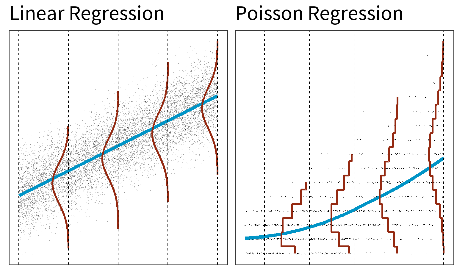
Gaussian response
Assume length is Gaussian with
\(Var(\epsilon) = \sigma^2\)
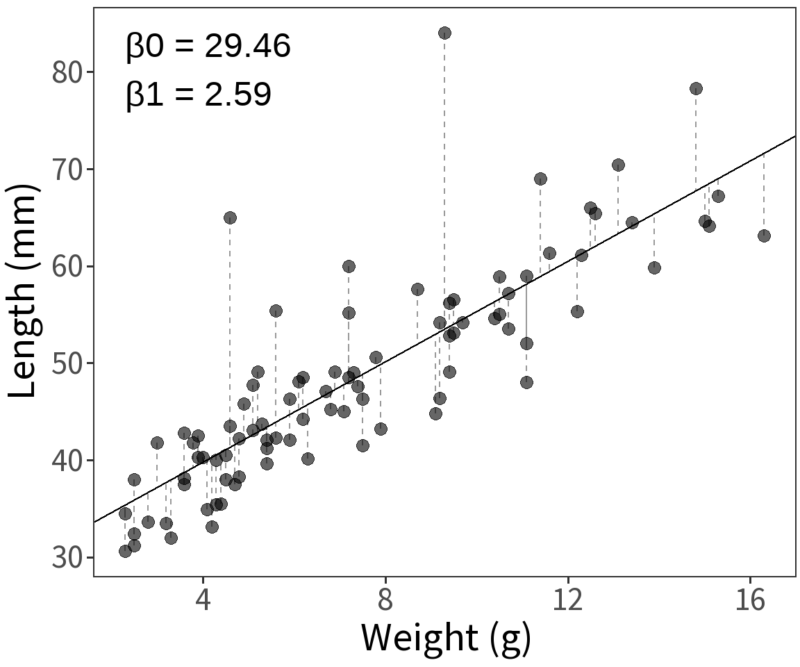
\(E(Y) = \mu = \beta X\)
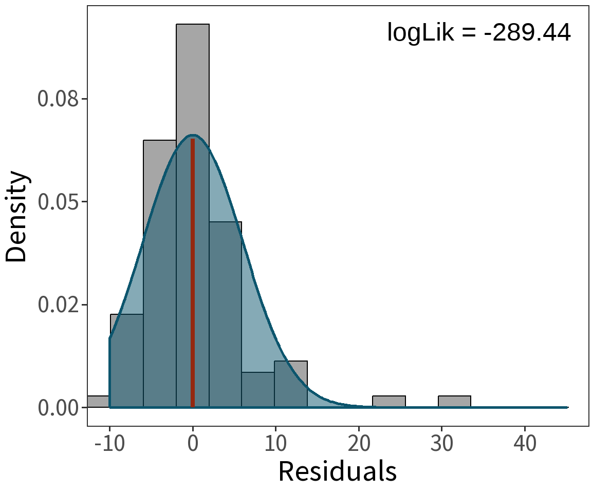
Question What is the probability that we observe these data given a model with parameters \(\beta\) and \(\sigma^2\)?
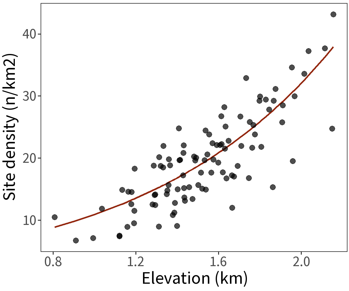
Poisson GLM
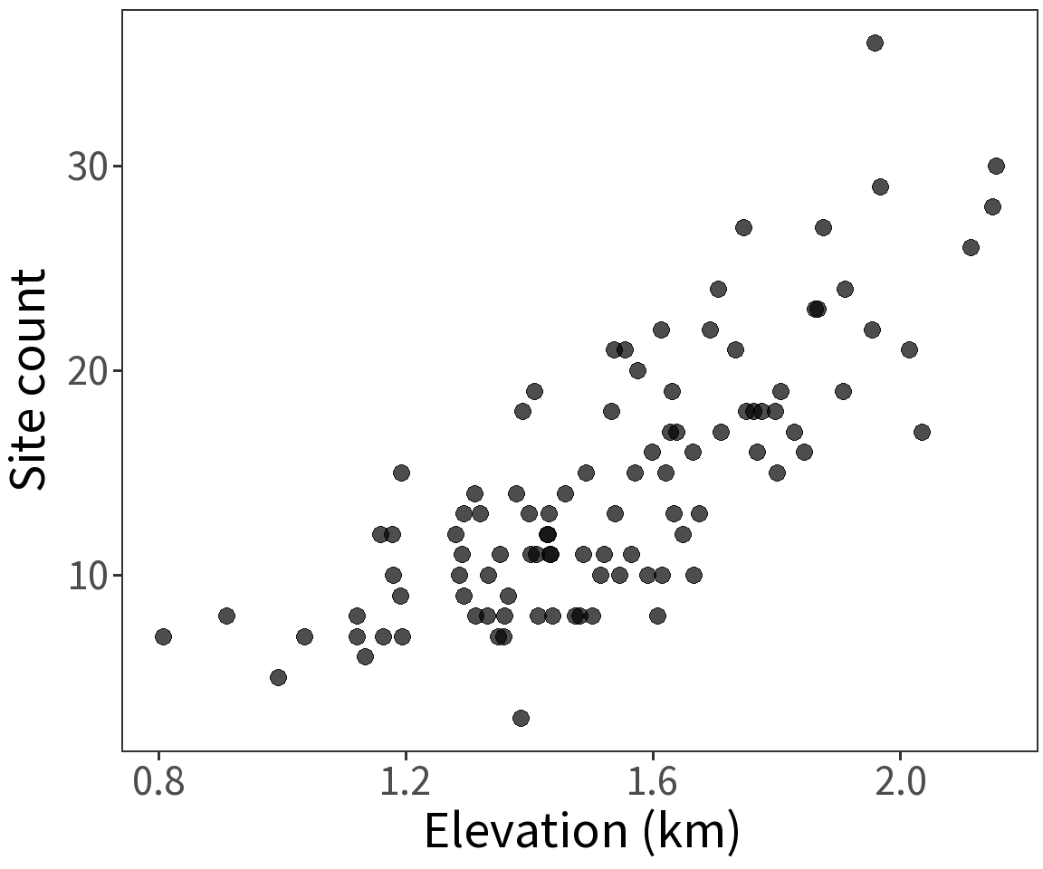
Counts arise from a Poisson process with expectation \(E(Y) = \lambda\) and
\[log\,\lambda = \beta X\]
By taking the log, this constrains the expected count to be greater than zero.
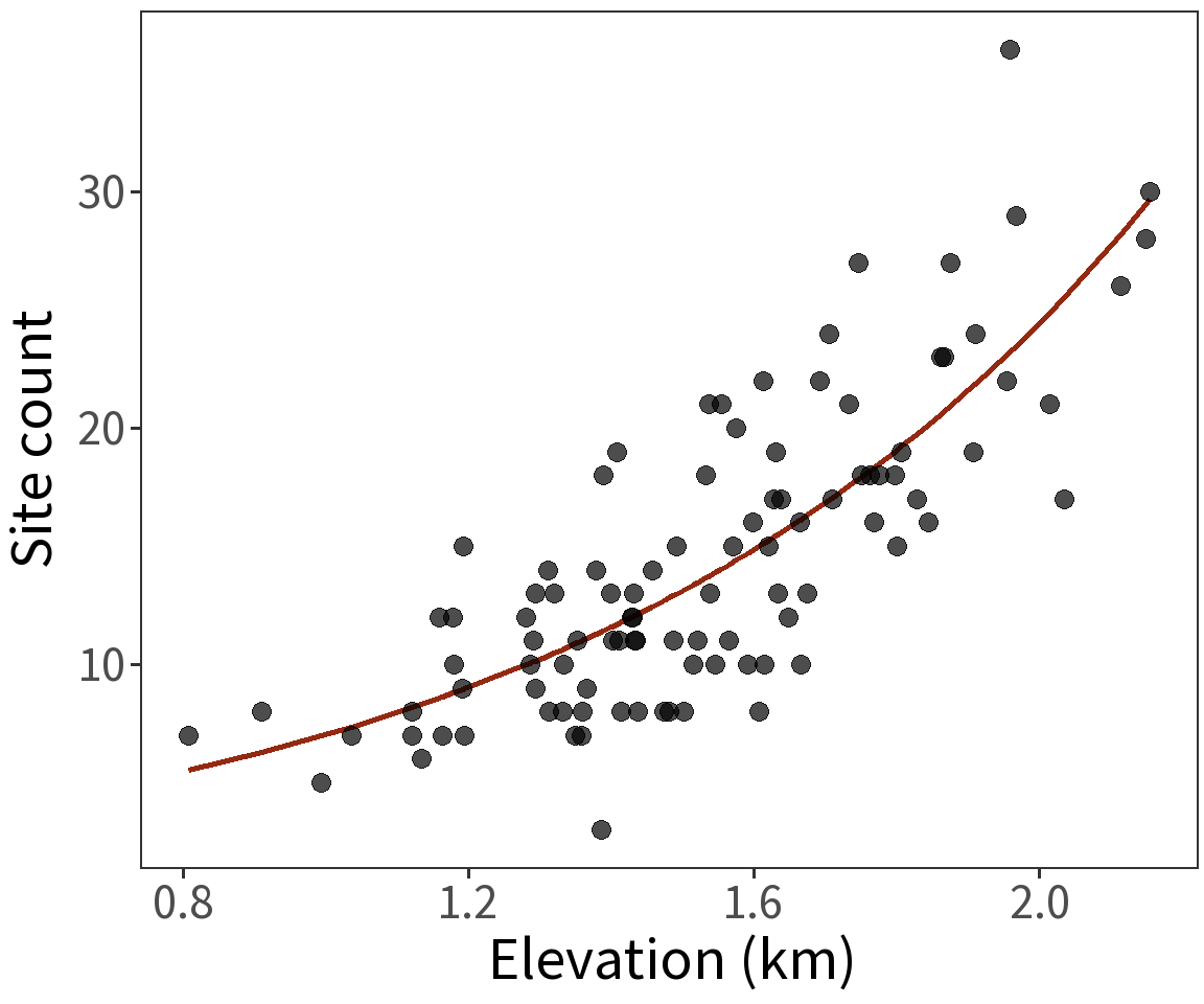
Estimated coefficients:
\(\beta_0 = 0.7074\)
\(\beta_1 = 1.2442\)
⚠️ Coefficients are on the log scale! To get counts, need the exponent.
\(\beta_0 = exp(0.7074) = 2.0286\)
\(\beta_1 = exp(1.2442) = 3.4701\)
For a one unit increase in elevation, the count of sites increases by 3.4701.
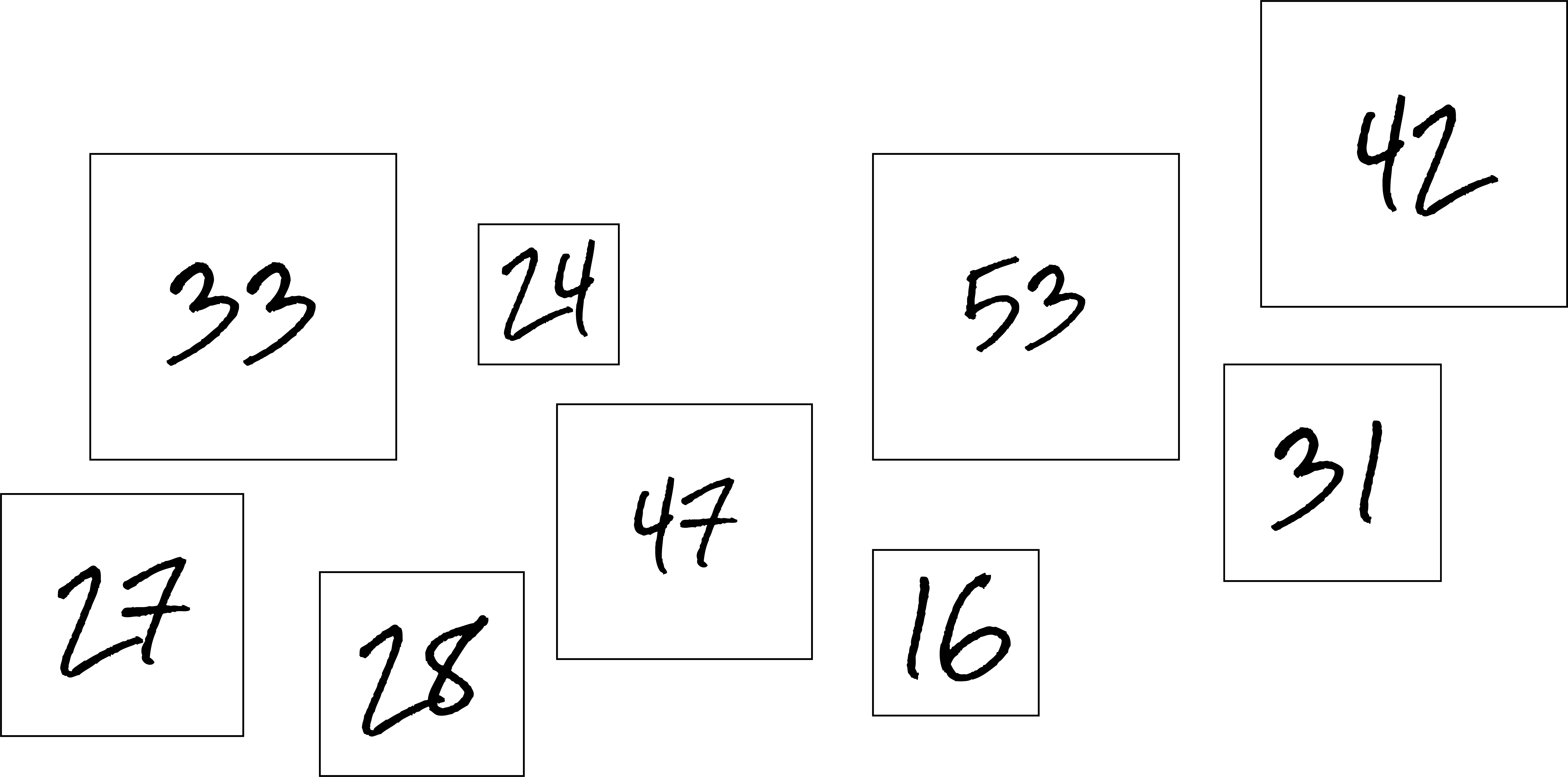
A count relative to what?
Survey blocks? Need to account for area in our sampling strategy!
Offset
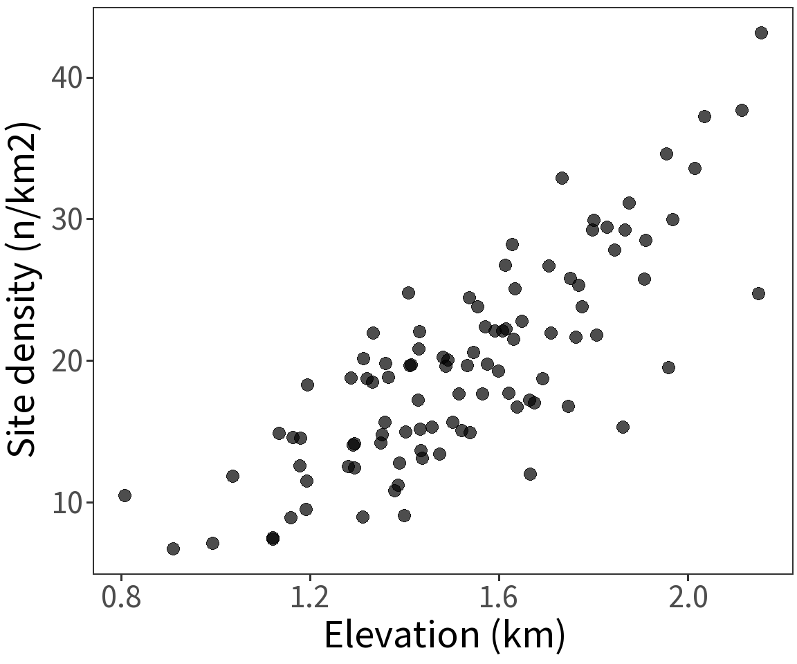
Model the density
\[log\;(\lambda_i/area_i) = \beta X\] Equivalent to
\[log\;(\lambda_i) = \beta X + log\;(area_i)\]
Still linear! Still modeling counts!

Estimated coefficients:
\(\beta_0 = 1.3899\)
\(\beta_1 = 1.0537\)
For these, the log Likelihood is
\(\mathcal{l} = -444.0432\)
Accounting for dispersion
Two strategies:
- quasi-Poisson
- negative binomial
⚠️ Trade-offs! QP doesn’t use MLE. NB can’t be fit with stats::glm().
| Est. | S.E. | t | p | |
|---|---|---|---|---|
| (Intercept) | 1.314 | 0.120 | 10.986 | <0.001 |
| elevation | 1.077 | 0.076 | 14.197 | <0.001 |