Lecture 12: Logistic Regression
3/28/23
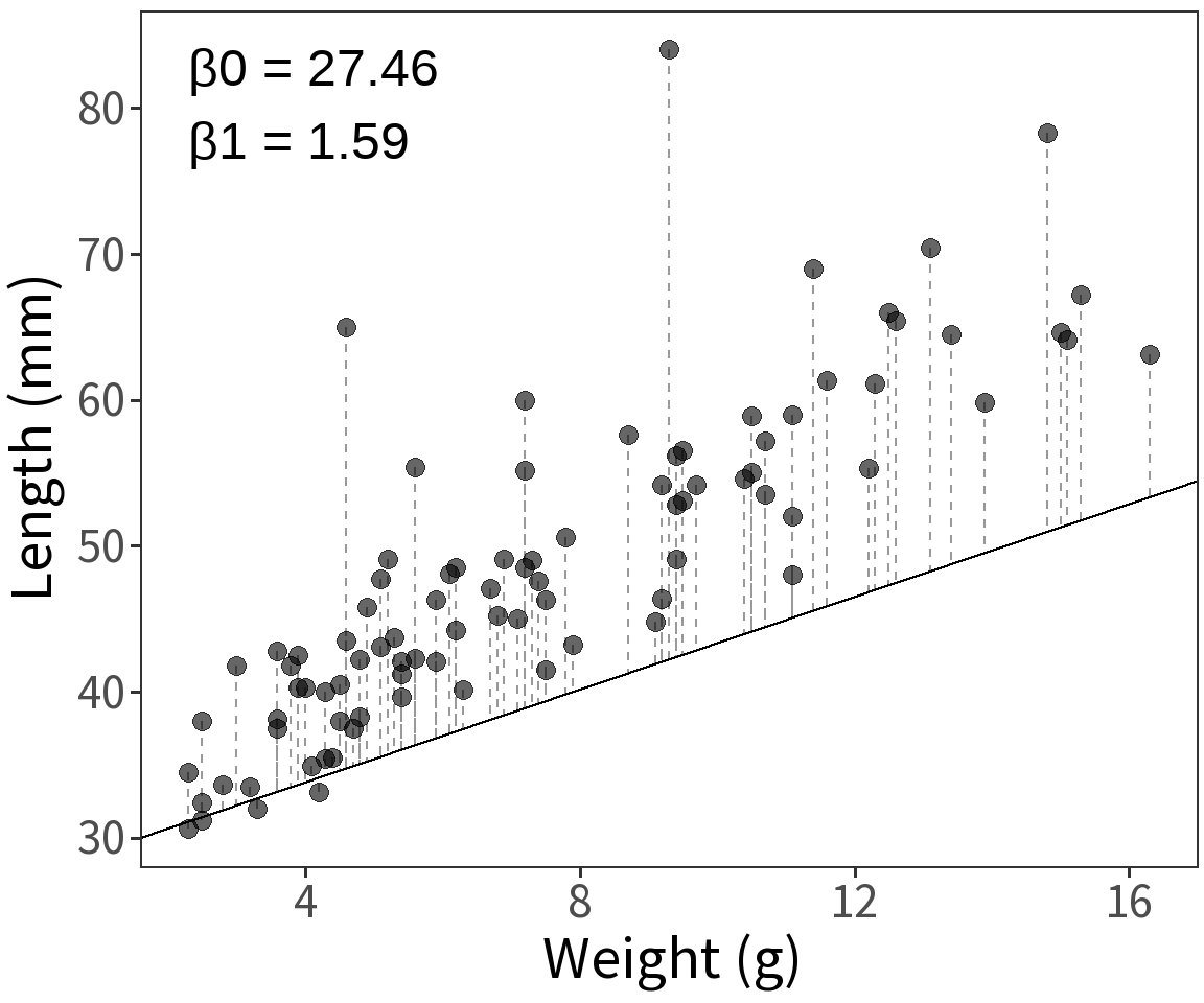
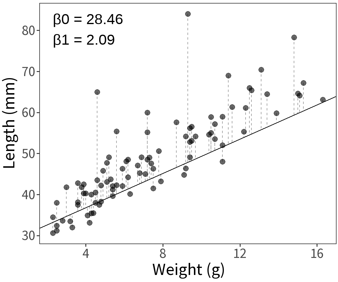
Gaussian response
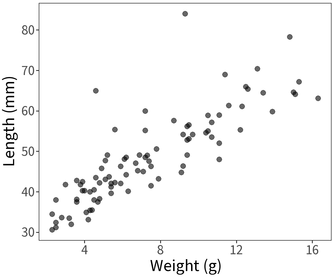
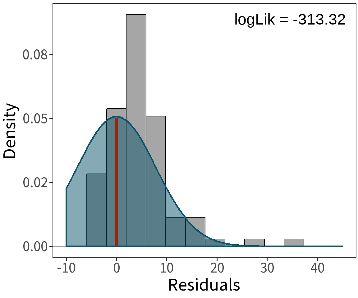
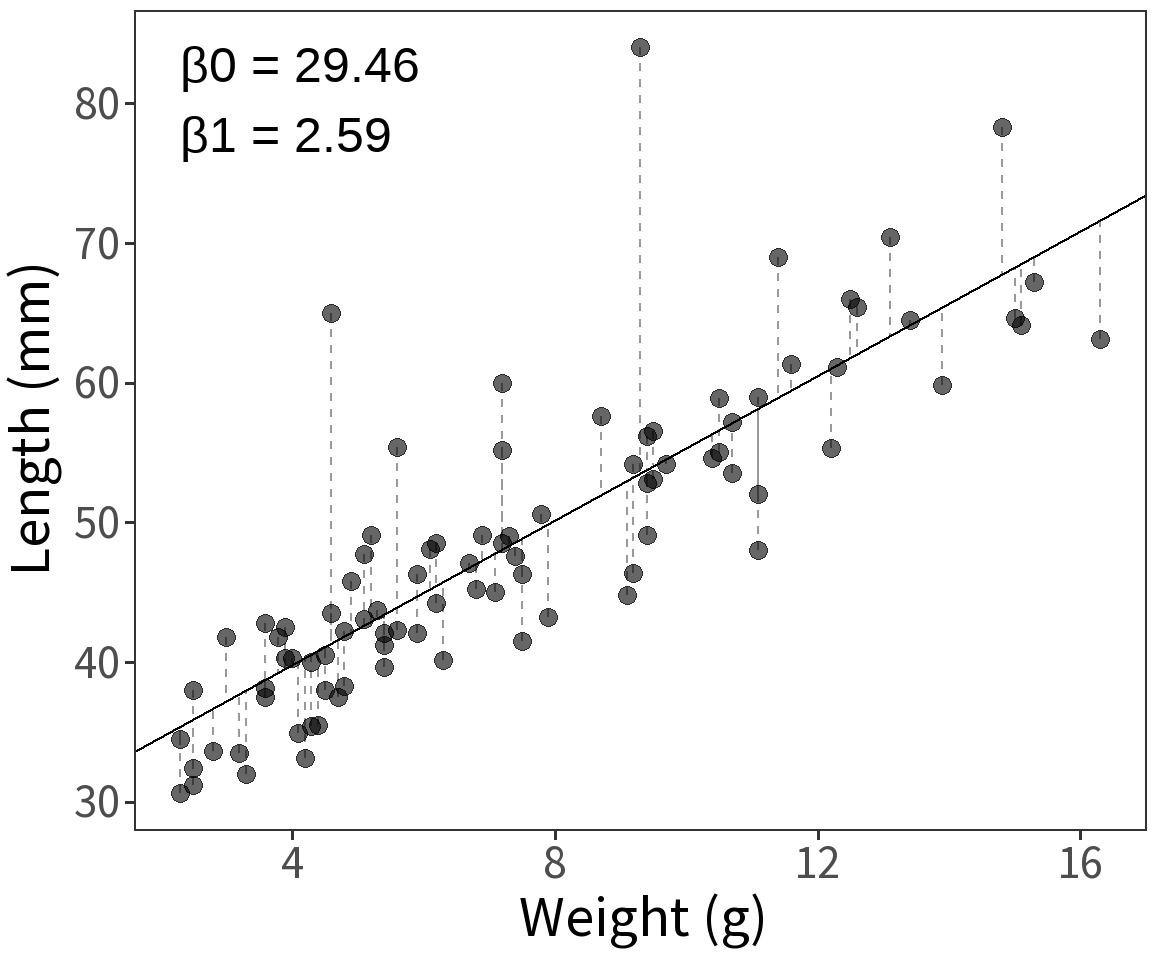
Assume length is Gaussian with
\(Var(\epsilon) = \sigma^2\)
\(E(Y) = \mu = \beta X\)
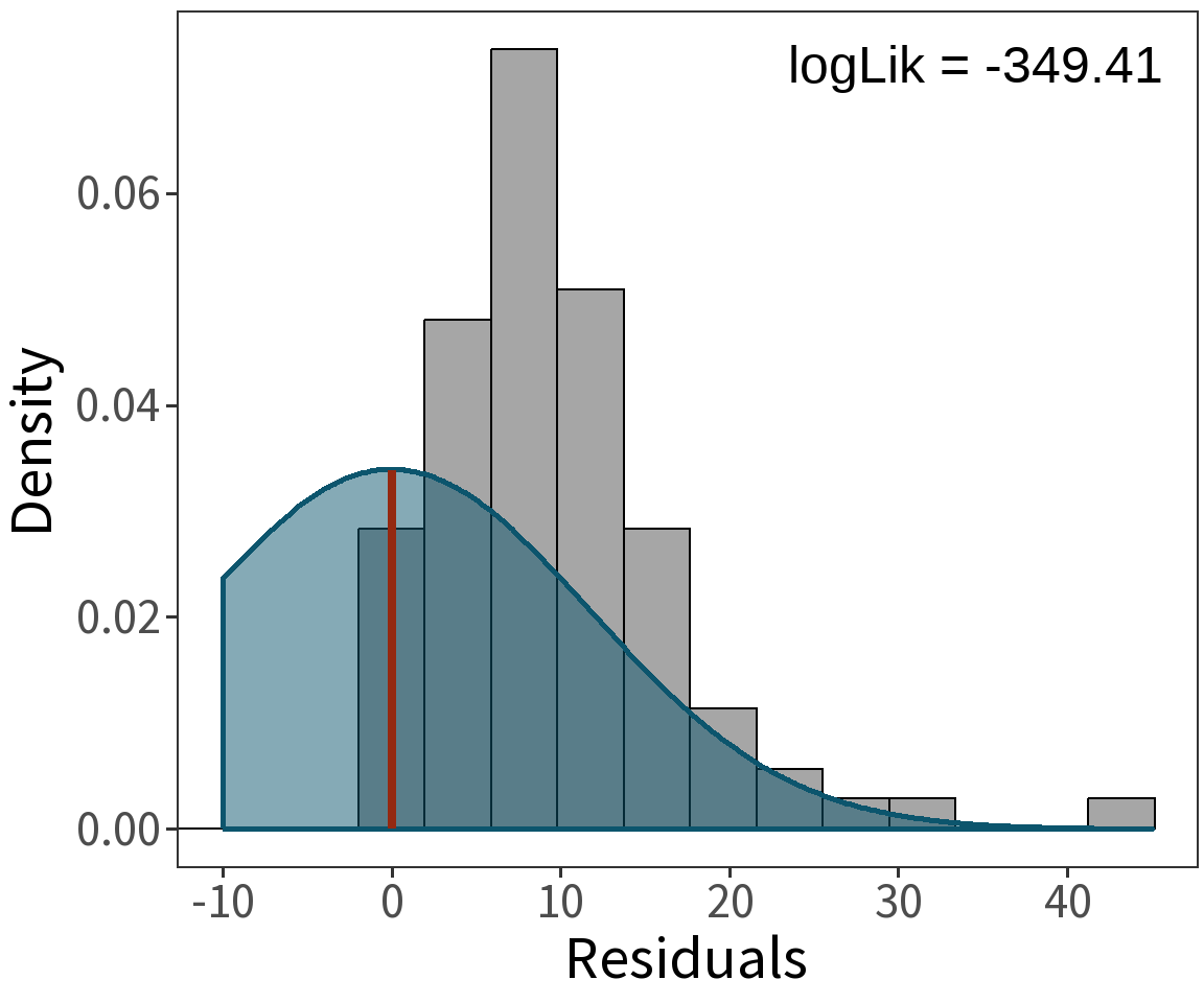
Question What is the probability that we observe these data given a model with parameters \(\beta\) and \(\sigma^2\)?
Bernoulli response
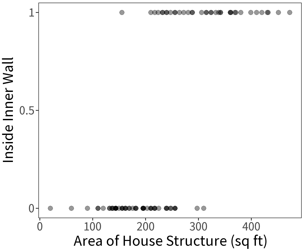
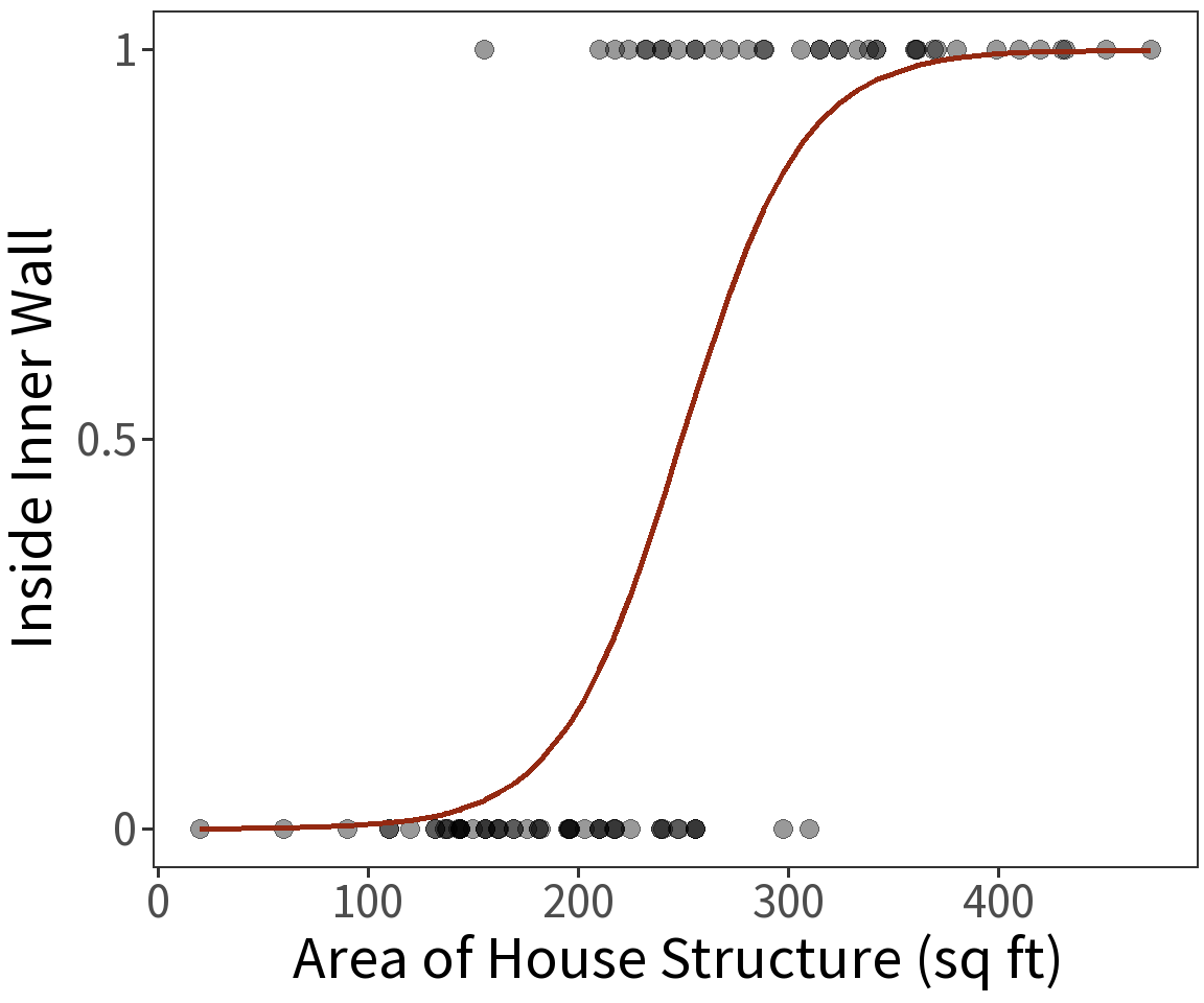
Location inside or outside of the inner wall at the Snodgrass site is a Bernoulli variable and has expectation \(E(Y) = p\) where
\[p = \frac{1}{1 + exp(-\beta X)}\] This defines a logistic curve or sigmoid, with \(p\) being the probability of success. This constrains the estimate \(E(Y)\) to be in the range 0 to 1.

Taking the log of \(p\) gives us
\[log(p) = log\left(\frac{p}{1 - p}\right) = \beta X\]
This is known as the “logit” or log odds.
Question What is the probability that we observe these data (these inside features) given a model with parameters \(\beta\)?
Estimated coefficients:
\(\beta_0 = -8.6631\)
\(\beta_1 = 0.0348\)
For these, the log Likelihood is
\(\mathcal{l} = -28.8641\)
Interpretation

Estimated coefficients:
\(\beta_0 = -8.6631\)
\(\beta_1 = 0.0348\)
Note that these coefficient estimates are log-odds! To get the odds, we take the exponent.
\(\beta_0 = exp(-8.6631) = 0.0002\)
\(\beta_1 = exp(0.0348) = 1.0354\)
For a one unit increase in area, the odds of being in the inside wall increase by 1.0354.
Estimated coefficients:
\(\beta_0 = -8.6631\)
\(\beta_1 = 0.0348\)
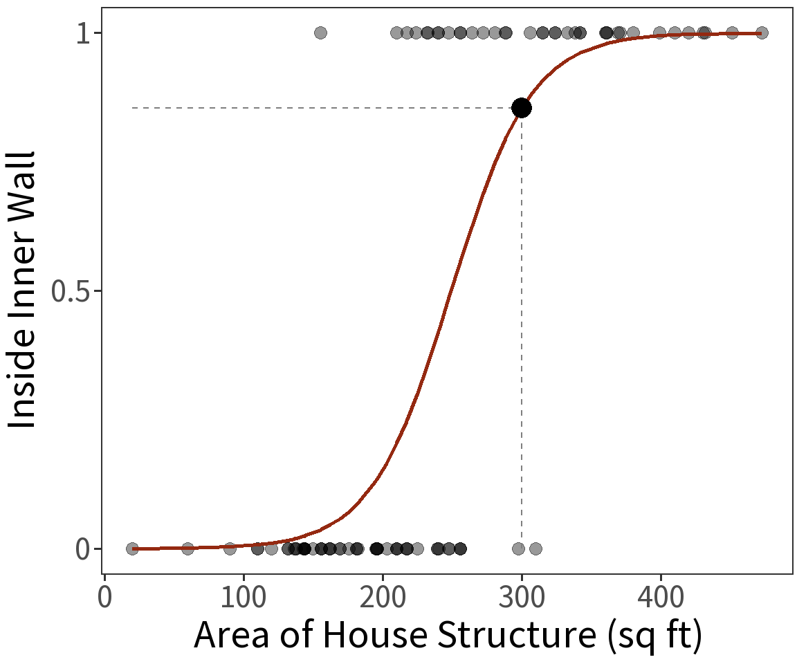
To get the probability, we can use the mean function (also known as the inverse link):
\[p = \frac{1}{1+exp(-\beta X)}\]
For a house structure with an area of 300 square feet, the estimated probability that it occurs inside the inner wall is 0.8538.
Proportional response
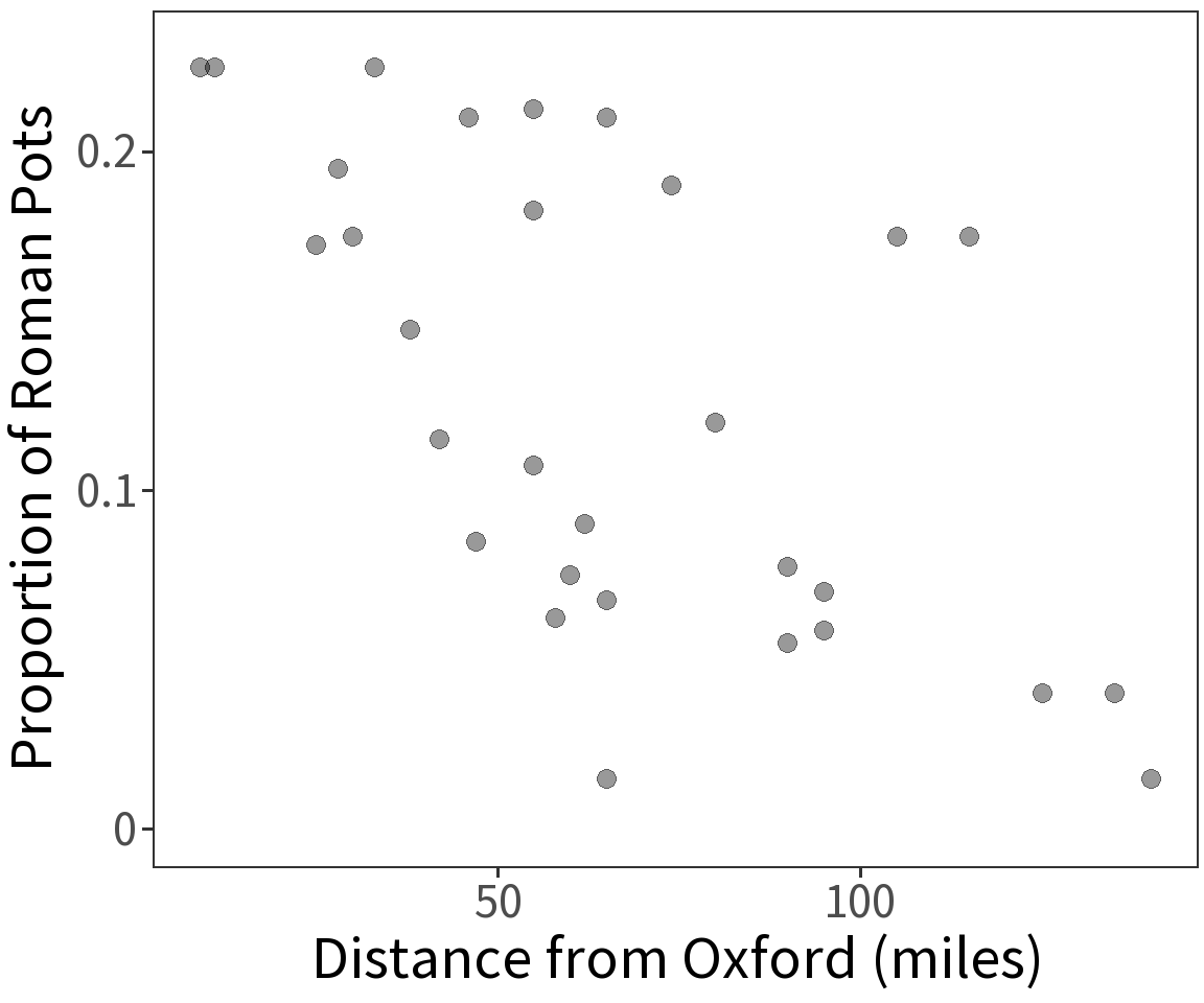
Proportion of Roman pottery is a binomial variable and has expectation \(E(Y) = p\) where
\[p = \frac{1}{1 + exp(-\beta X)}\] This defines a logistic curve or sigmoid, with \(p\) being the proportion of successful Bernoulli trials. This constrains the estimate \(E(Y)\) to be in the range 0 to 1.

Taking the log of \(p\) gives us
\[log(p) = log\left(\frac{p}{1 - p}\right) = \beta X\]
This is known as the “logit” or log odds.
Question What is the probability that we observe these data (these proportions) given a model with parameters \(\beta\)?
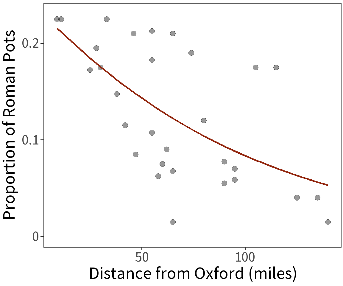
Estimated coefficients:
\(\beta_0 = -1.1818\)
\(\beta_1 = -0.0121\)
For these, the log Likelihood is
\(\mathcal{l} = -4.1148\)