Lecture 07: Evaluating Linear Models
2/21/23
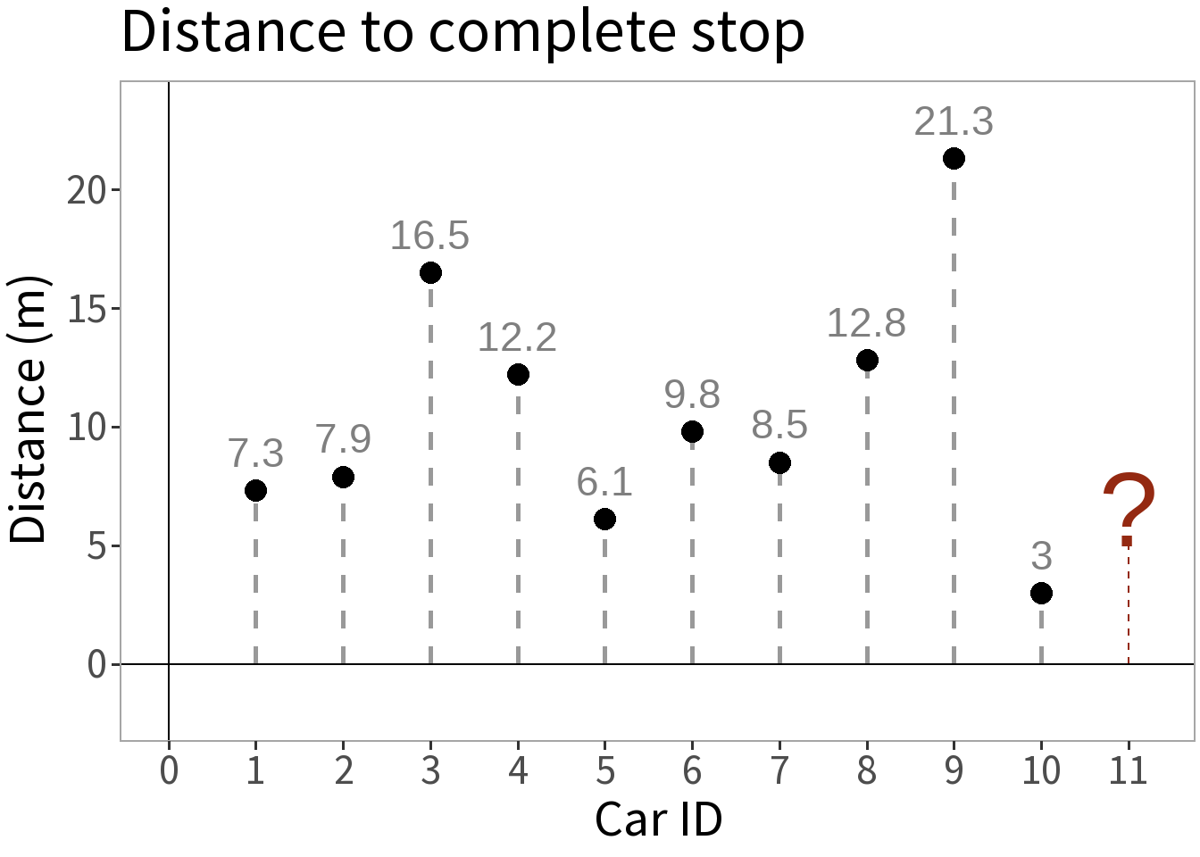
Competing Models
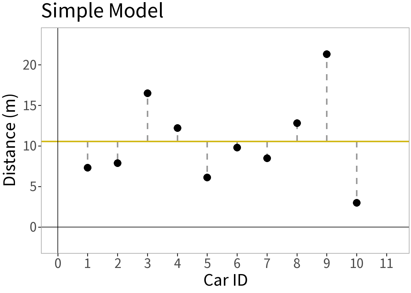
E[Y]: mean distance
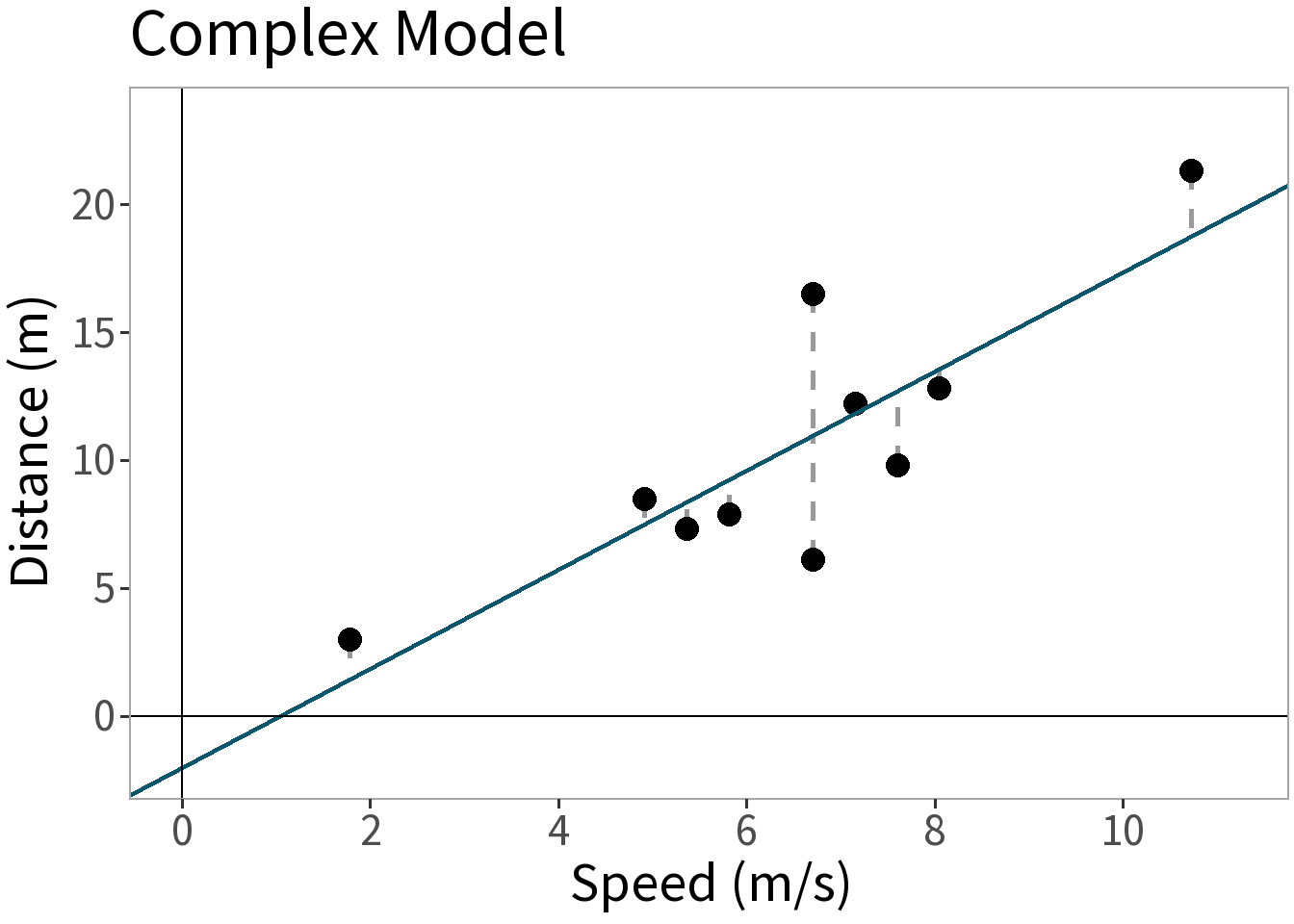
E[Y]: some function of speed]
Model Formula
\[ \begin{align} y_i &= E[Y] + \epsilon_i \\ \epsilon &\sim N(0,\sigma) \\ \sigma &= 2.91 \end{align} \]
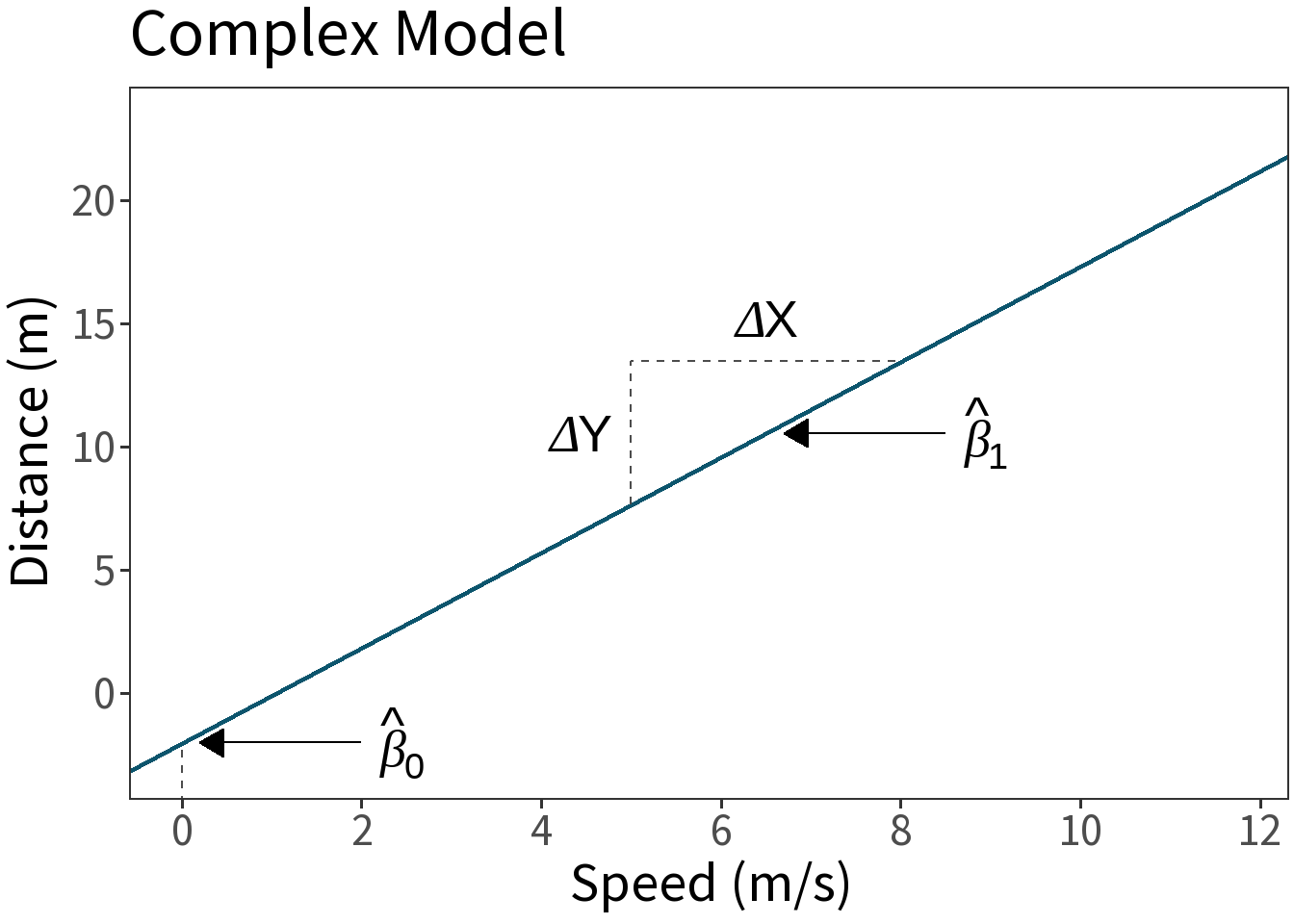
\[ \begin{align} E[Y] &\approx \hat\beta X \\ \hat\beta_0 &= -2.01 \\ \hat\beta_1 &= 1.94 \end{align} \]
\(\hat\beta_{0}\) is the value of \(Y\) where \(X=0\), here the total stopping distance when the car isn’t moving, which should be zero!!!
\(\hat\beta_{1}\) is change in \(Y\) relative to change in \(X\), here the additional distance the car will travel for each unit increase in speed.
Prediction

\[ \begin{align} y_i &= E[Y] + \epsilon_i \\ \epsilon &\sim N(0,\sigma) \\ \sigma &= 2.91 \end{align} \]
\[ \begin{align} E[Y] &\approx \hat\beta X \\ \hat\beta_0 &= -2.01 \\ \hat\beta_1 &= 1.94 \end{align} \]
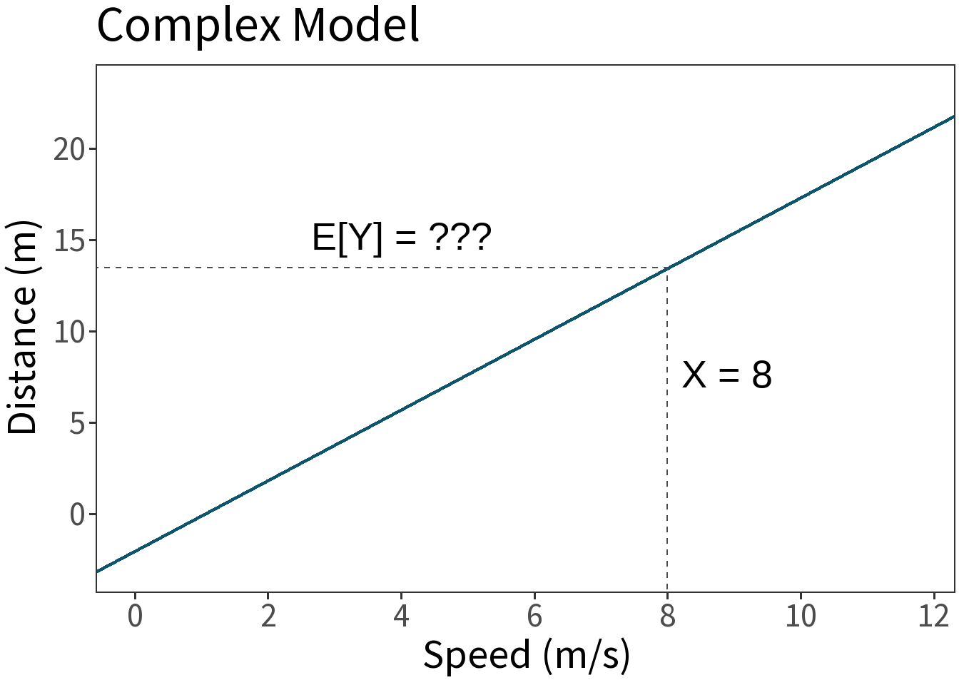
Question: if a car is going 8 m/s when it applies the brakes, how long will it take it to stop?
\[ E[Y] = -2.01 + 1.94 \cdot 8 = 13.48 \]
Prediction Interval

\[ \begin{align} y_i &= E[Y] + \epsilon_i \\ \epsilon &\sim N(0,\sigma) \\ \sigma &= 2.91 \end{align} \]
\[ \begin{align} E[Y] &\approx \hat\beta X \\ \hat\beta_0 &= -2.01 \\ \hat\beta_1 &= 1.94 \end{align} \]
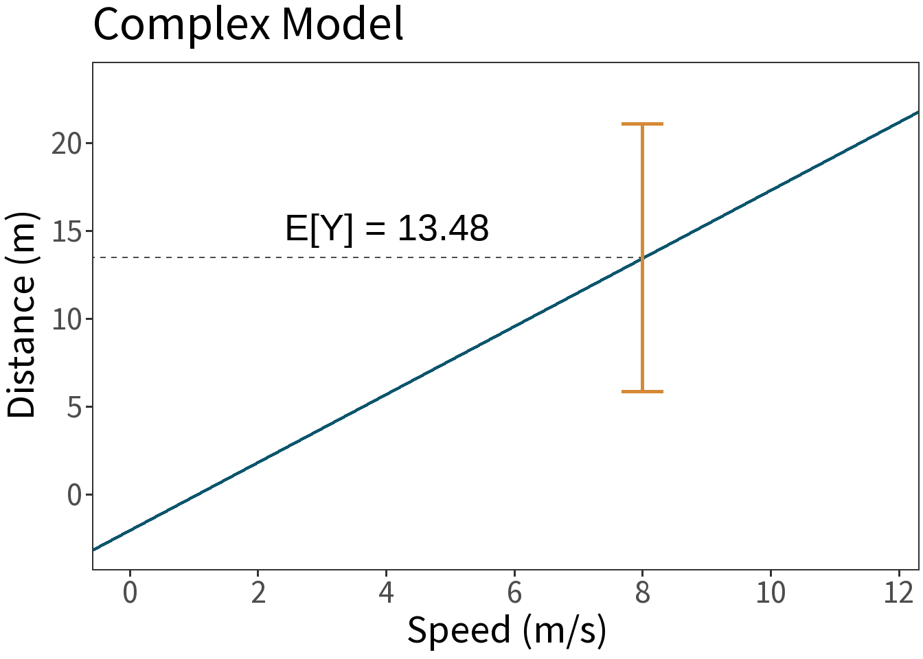
Question: But, what about \(\epsilon\)?!!!
We can visualize this with a prediction interval, or the range within which a future outcome is expected to fall with a certain probability for some value of \(X\). Can generalize this outside the range of the model, but with increasing uncertainty.
Confidence Interval

\[ \begin{align} y_i &= E[Y] + \epsilon_i \\ \epsilon &\sim N(0,\sigma) \\ \sigma &= 2.91 \end{align} \]
\[ \begin{align} E[Y] &\approx \hat\beta X \\ \hat\beta_0 &= -2.01 \\ \hat\beta_1 &= 1.94 \end{align} \]
Question: But, what if we’re wrong about \(\beta\)?!!!
We can visualize this with a confidence interval, or the range within which the average outcome is expected to fall with a certain probability for some value of \(X\).
Model Complexity
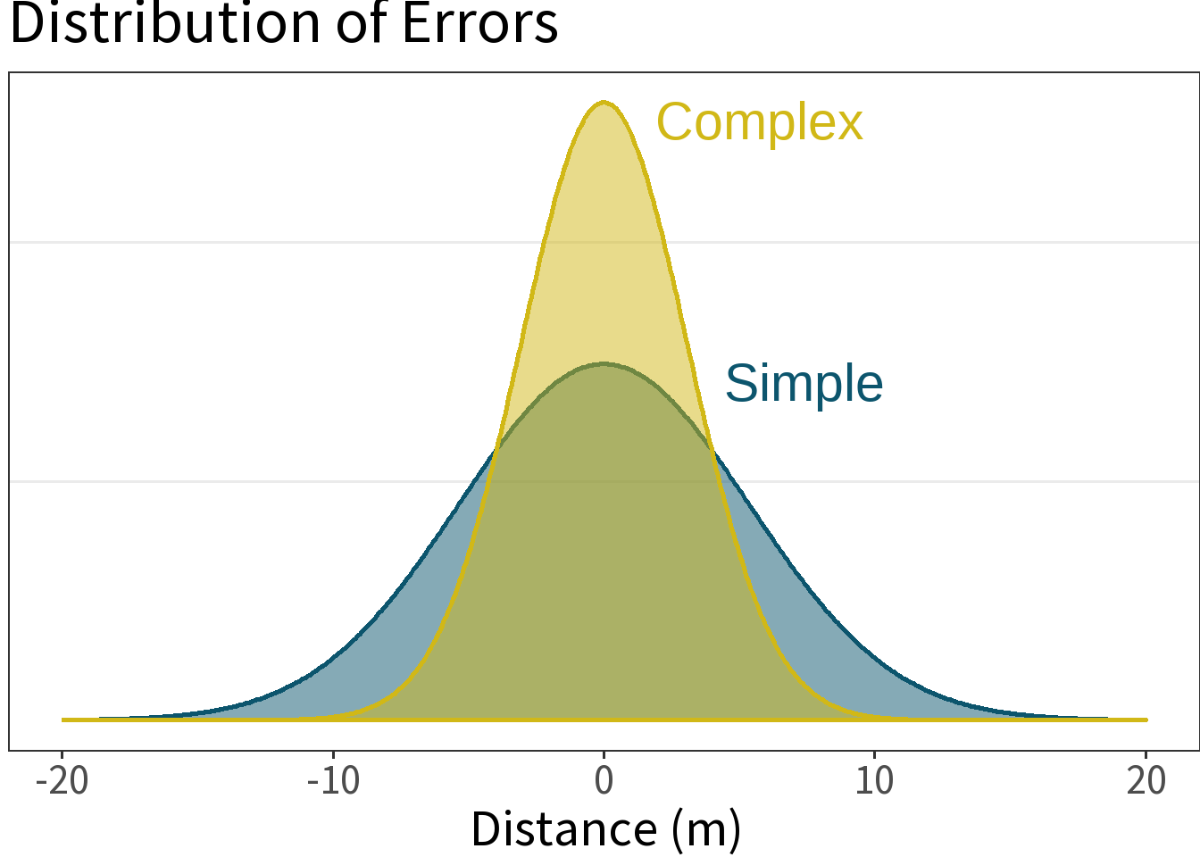
⚖️ The error is smaller for the more complex model. This is a good thing, but what did it cost us? Need to weigh this against the increased complexity!
ANOVA for model
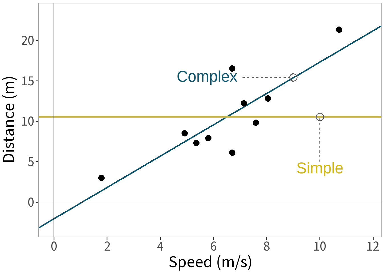
We have two models of our data, one simple, the other complex.
Question: Does the complex (bivariate) model explain more variance than the simple (intercept) model? Does the difference arise by chance?
The null hypothesis:
- \(H_0:\) no difference in variance explained.
The alternate hypothesis:
- \(H_1:\) difference in variance explained.
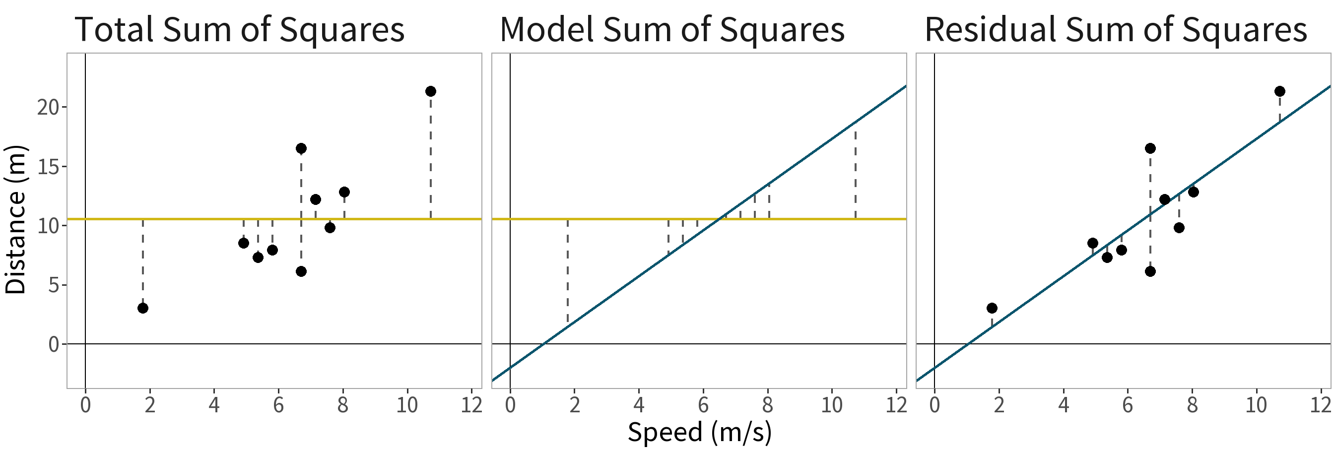
Variance Decomposition. Total variance in the dependent variable can be decomposed into the variance captured by the more complex model and the remaining (or residual) variance:
Decompose the differences:
\((y_{i} - \bar{y}) = (\hat{y}_{i} - \bar{y}) + (y_{i} - \hat{y}_{i})\)
where
- \((y_{i} - \bar{y})\) is the total error,
- \((\hat{y}_{i} - \bar{y})\) is the model error, and
- \((y_{i} - \hat{y}_{i})\) is the residual error.
Sum and square the differences:
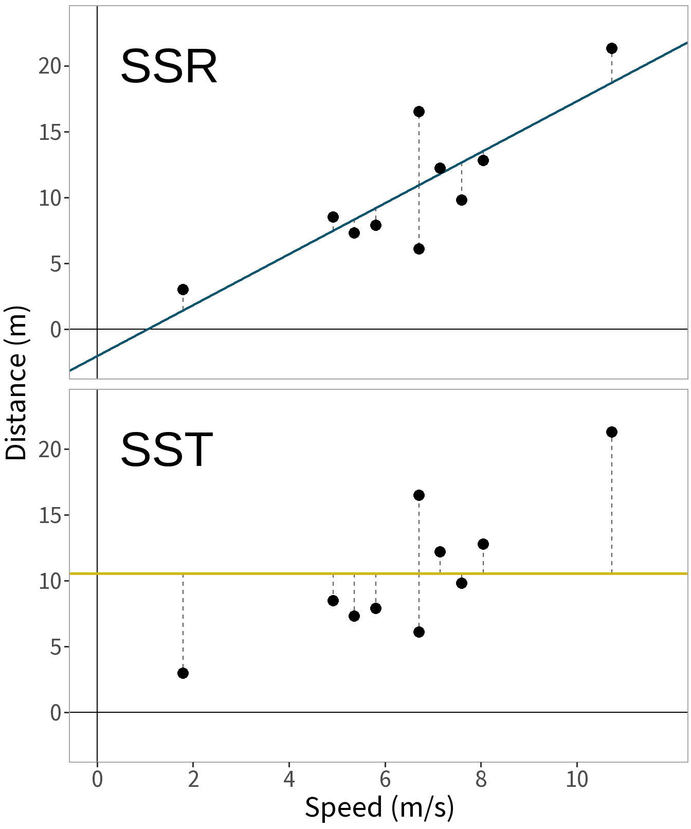
\(SS_{T} = SS_{M} + SS_{R}\)
where
- \(SS_{T}\): Total Sum of Squares
- \(SS_{M}\): Model Sum of Squares
- \(SS_{R}\): Residual Sum of Squares
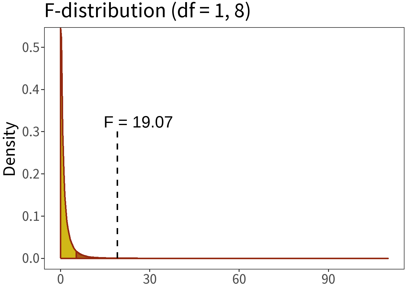
\[F = \frac{\text{model variance}}{\text{residual variance}}\]
where
Model variance = \(SS_{M}/k\) for \(k\) model parameters
Residual variance = \(SS_{R}/(n-k-1)\) for \(k\) and \(n\) observations.
Question: How probable is it that \(F=\) 19.07?
We can answer this by comparing the F-statistic to the F-distribution.
Summary:
- \(\alpha = 0.05\)
- \(H_0:\) no difference
- \(p=\) 0.0024
Translation: the null hypothesis is really, really unlikely. So, there must be some difference between models!
R-Squared
Coefficient of Determination
\[R^2 = 1- \frac{SS_{R}}{SS_{T}}\]
- Proportion of variance in \(y\) explained by the model \(M\).
- Scale is 0 to 1. A value closer to 1 means that \(M\) explains more variance.
- \(M\) is evaluated relative to simple, intercept-only model.
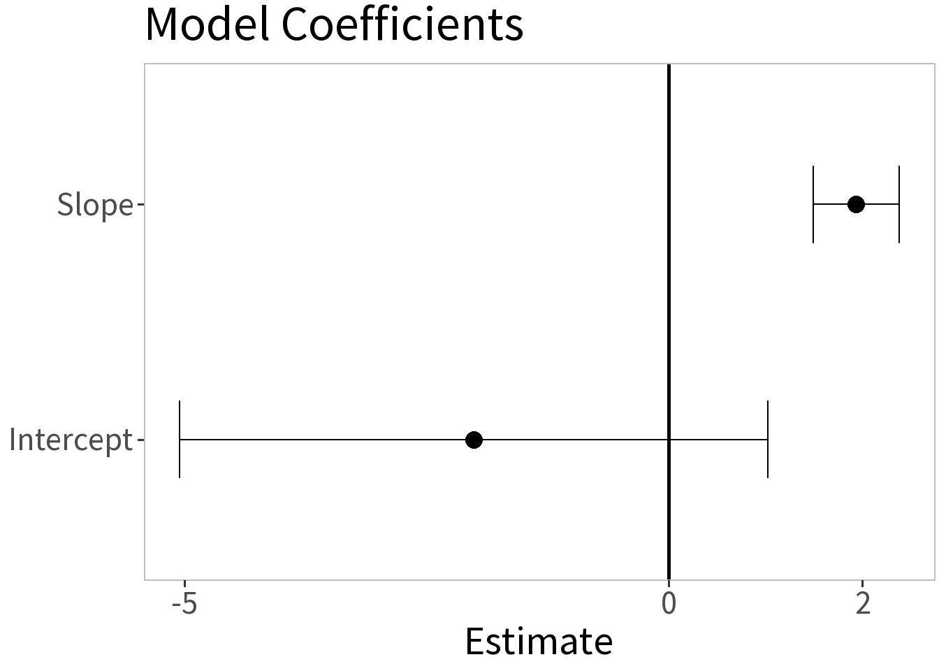
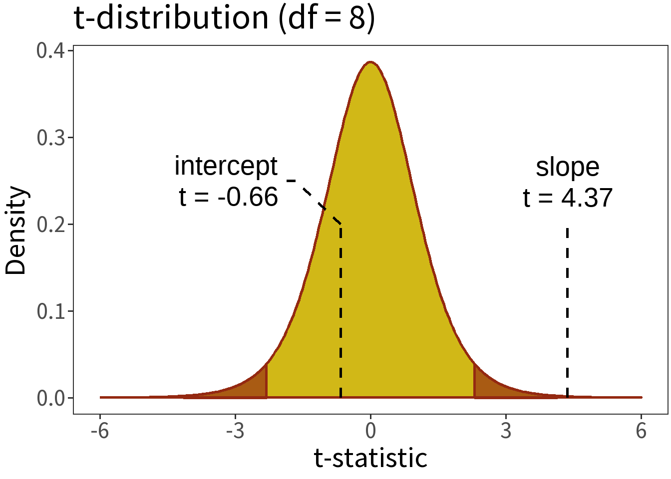
t-test for coefficients

Question: Are the coefficient estimates significantly different than zero?
To answer this question, we need some measure of uncertainty for these estimates.
The null hypothesis:
- \(H_0:\) coefficient estimate is not different than zero.
The alternate hypothesis:
- \(H_1:\) coefficient estimate is different than zero.
For simple linear regression,
the standard error of the slope, \(se(\hat\beta_1)\), is the ratio of the average squared error of the model to the total squared error of the predictor.
the standard error of the intercept, \(se(\hat\beta_0)\), is \(se(\hat\beta_1)\) weighted by the average squared values of the predictor.
The t-statistic is the coefficient estimate divided by its standard error
\[t = \frac{\hat\beta}{se(\hat\beta)}\]
This can be compared to a t-distribution with \(n-k-1\) degrees of freedom (\(n\) observations and \(k\) independent predictors).
Summary:
- \(\alpha = 0.05\)
- \(H_0\): \(\beta=0\)
- p-values:
- intercept = 0.5263
- slope < 0.0024
Diagnostic Plots
Weak Exogeneity: the predictor variables have fixed values and are known.
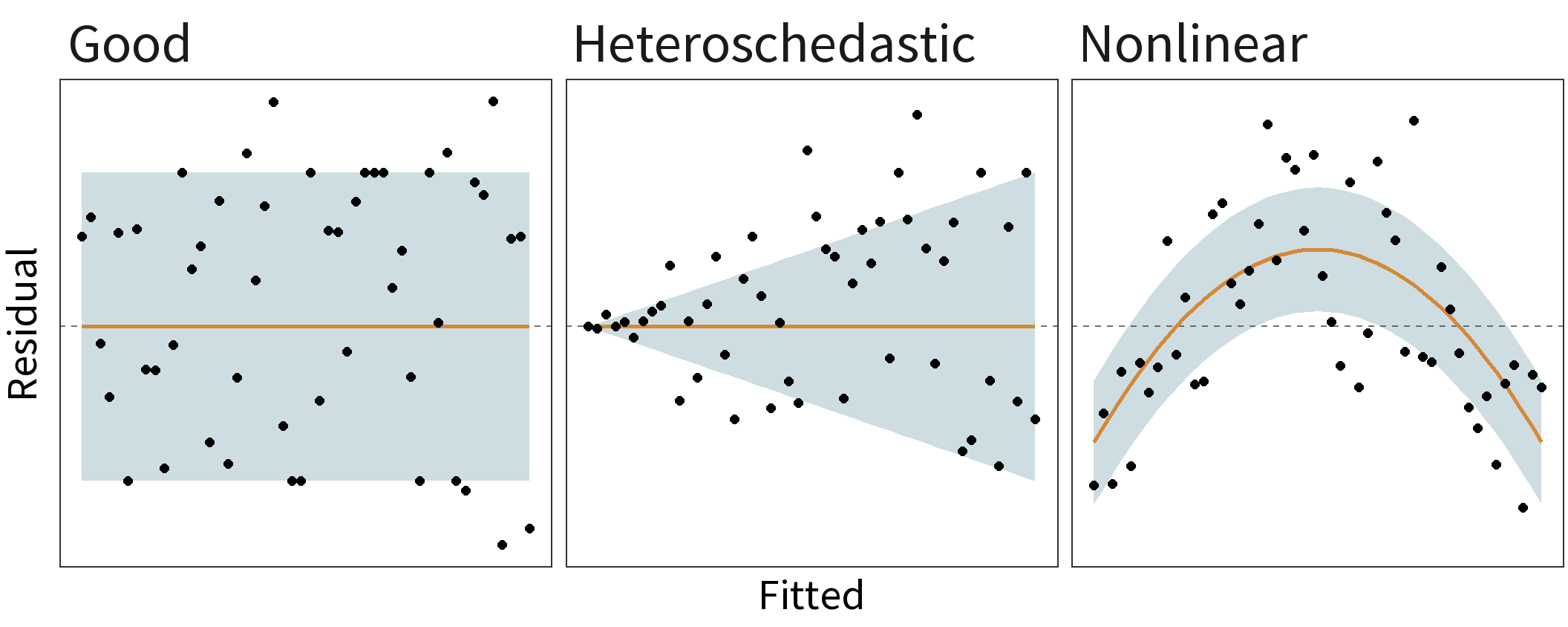
Linearity: the relationship between the predictor variables and the response variable is linear.
Constant Variance: the variance of the errors does not depend on the values of the predictor variables. Also known as homoscedasticity.
Independence of errors: the errors are uncorrelated with each other.
No perfect collinearity: the predictors are not linearly correlated with each other.