Lecture 04: Ordinary Least Squares
1/30/23
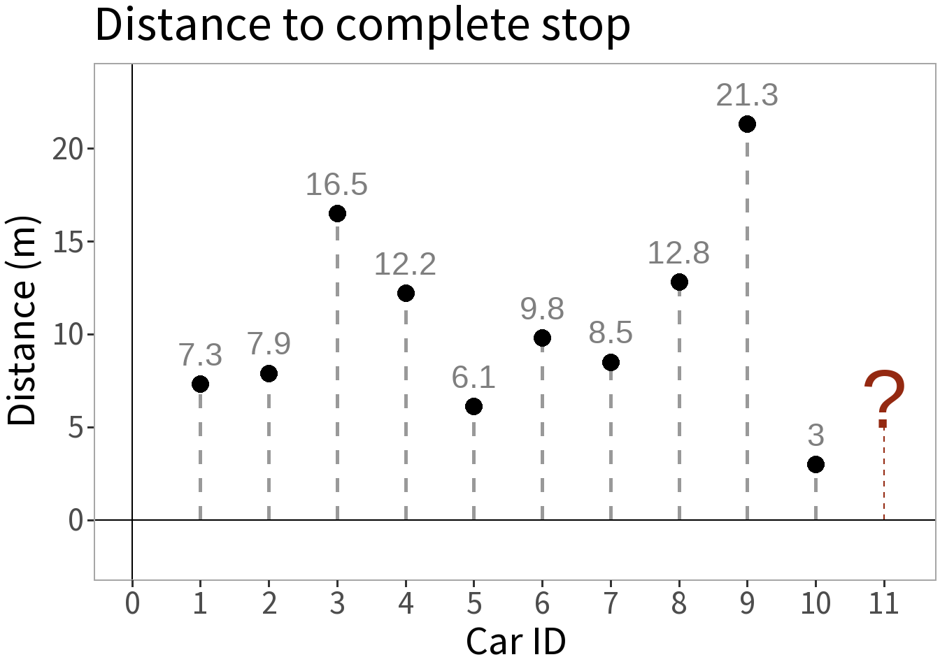
Competing Models
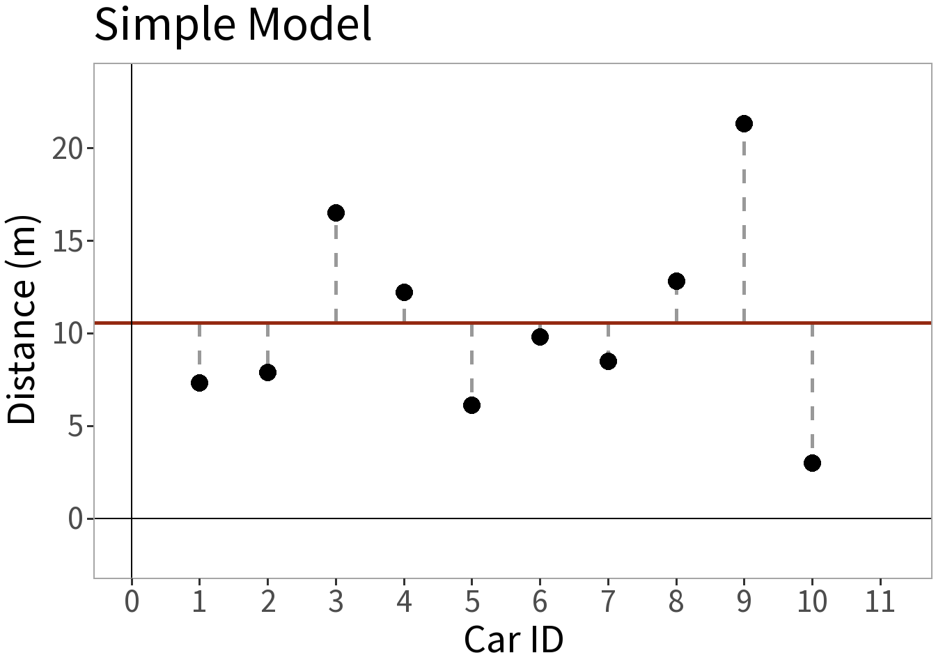
E[Y]: mean distance

E[Y]: some function of speed
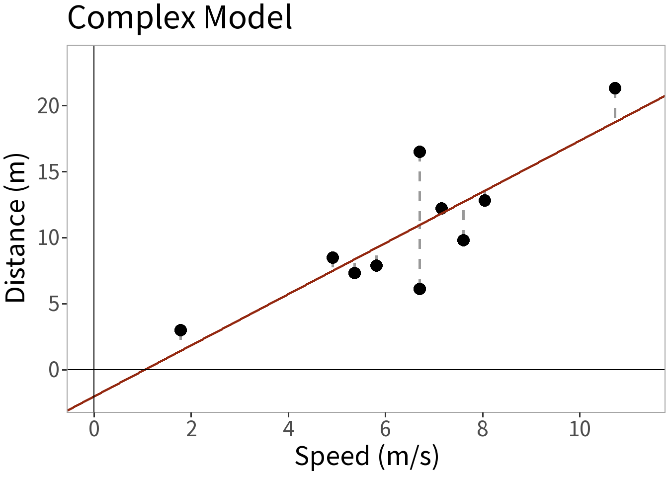
Model Complexity
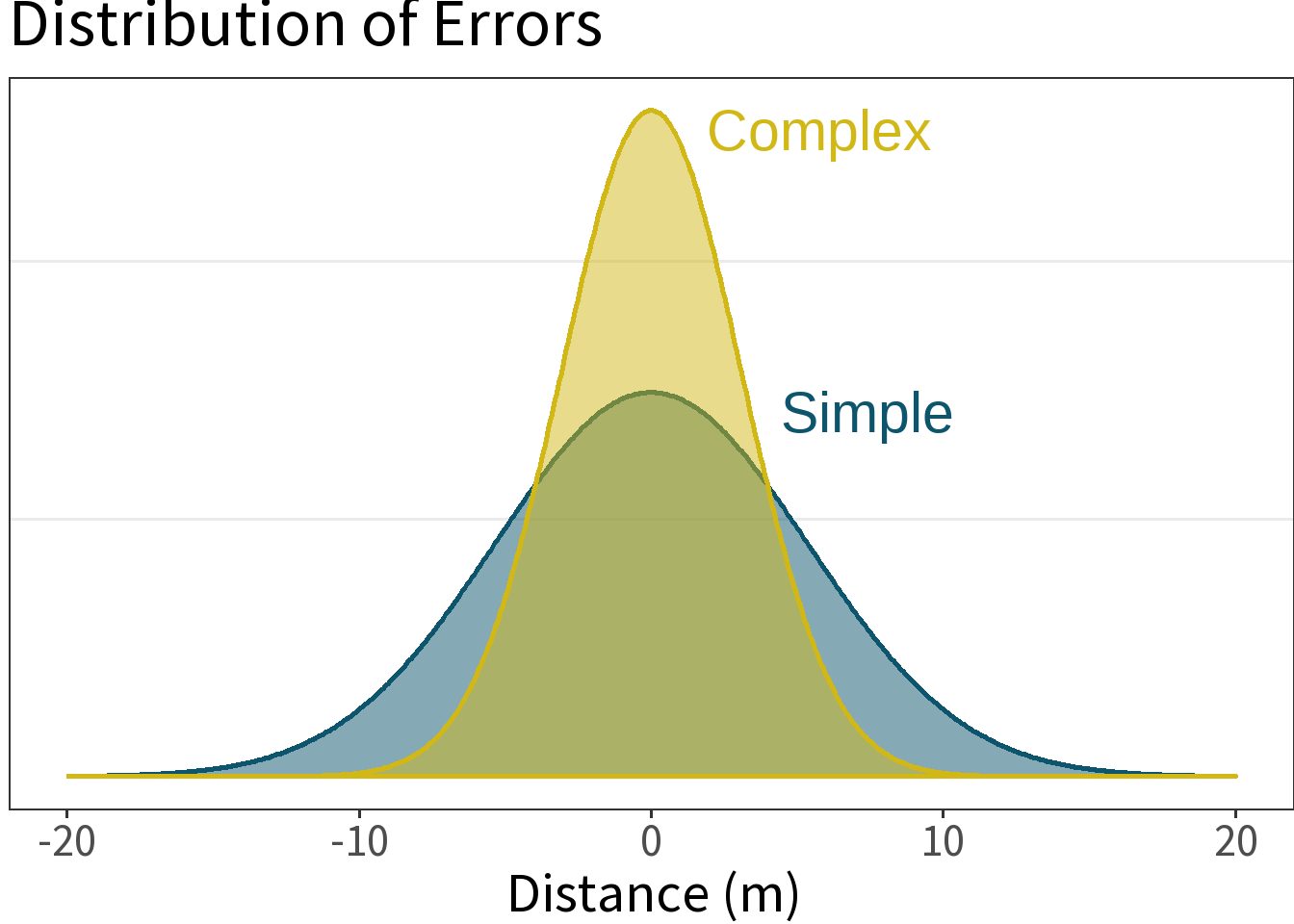
⚖️ The error is smaller for the more complex model. This is a good thing, but what did it cost us? Need to weigh this against the increased complexity!
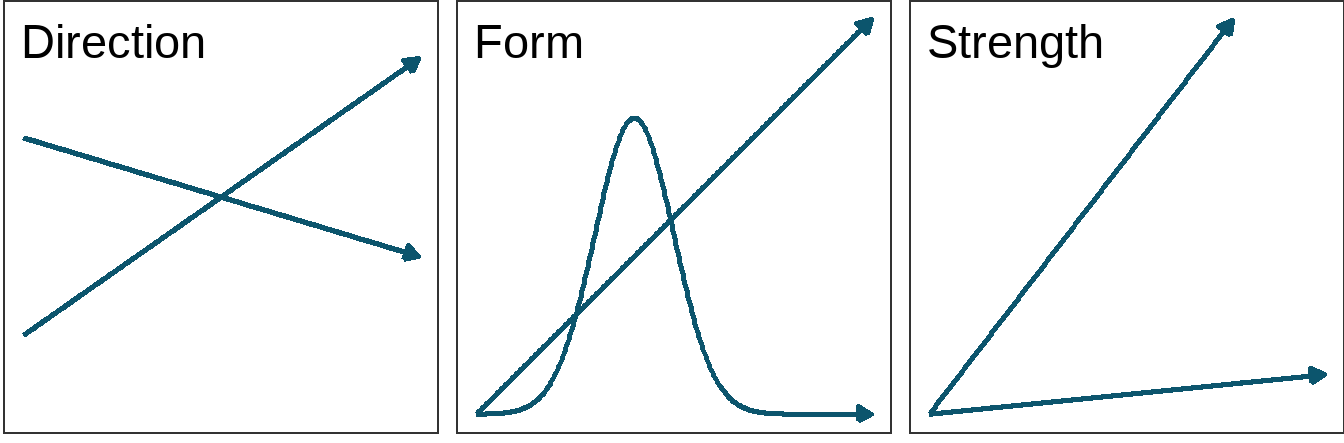
Bivariate statistics
Explore the relationship between two variables:
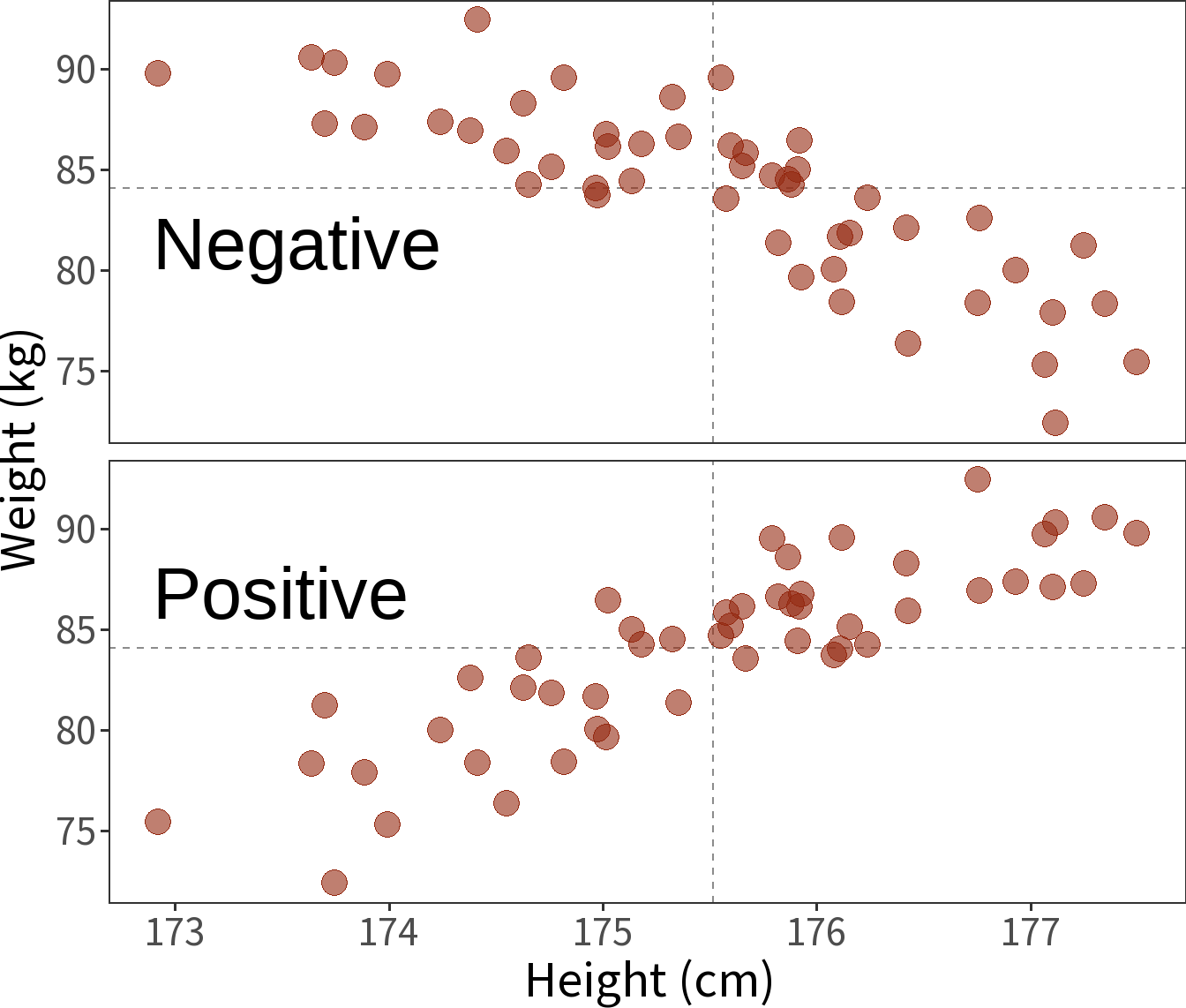
Covariance
The extent to which two variables vary together.
\[cov(x, y) = \frac{1}{n-1} \sum_{i=1}^{n} (x_i - \bar{x})(y_i - \bar{y})\]
- Sign reflects positive or negative trend, but magnitude depends on units (e.g., \(cm\) vs \(km\)).
- Variance is the covariance of a variable with itself.
Correlation
Pearson’s Correlation Coefficient
\[r = \frac{cov(x,y)}{s_{x}s_y}\]
Scales covariance (from -1 to 1) using standard deviations, \(s\), thus making magnitude independent of units.
Significance can be tested by converting to a t-statistic and comparing to a t-distribution with \(df=n-2\).

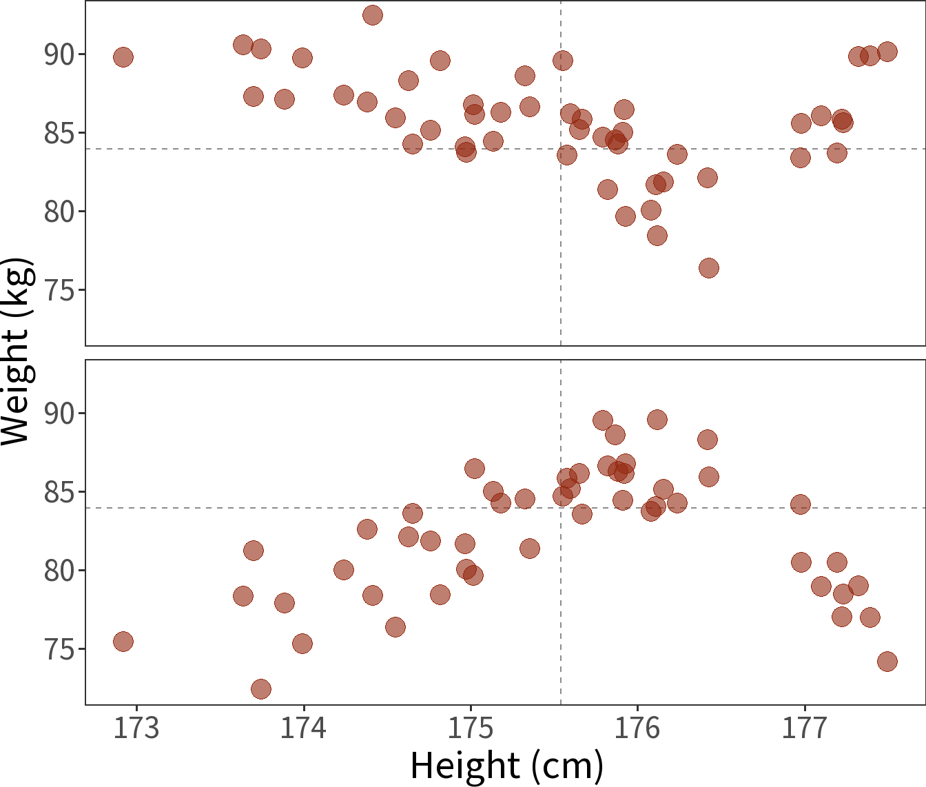
Non-linear correlation
Spearman’s Rank Correlation Coefficient
\[\rho = \frac{cov\left(R(x),\; R(y) \right)}{s_{R(x)}s_{R(y)}}\]
- Pearson’s correlation but with ranks (R).
- This makes it a robust estimate, less sensitive to outliers.
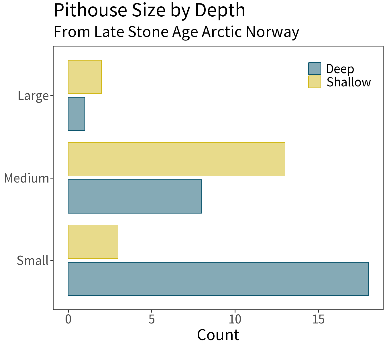
Correlation between categories
For counts or frequencies
\[\chi^2 = \sum \frac{(O_{ij}-E_{ij})^2}{E_{ij}}\]
- Analysis of contingency table
- \(O_{ij}\) is observed count in row \(i\), column \(j\)
- \(E_{ij}\) is expected count in row \(i\), column \(j\)
- Significance can be tested by comparing to a \(\chi^2\)-distribution with \(df=k-1\) (\(k\) being the number of categories).
Correlation is not causation!
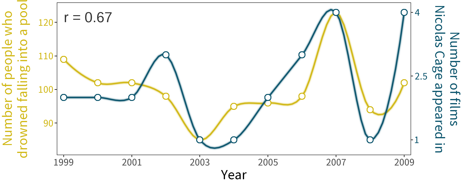
Adapted from https://www.tylervigen.com/spurious-correlations
Simple Linear Regression

‘Simple’ means one explanatory variable (speed)
\[y_i = \hat\beta_0 + \hat\beta_1 speed_i + \epsilon_i\]
- \(\hat\beta_0\) = -2.0107
- \(\hat\beta_1\) = 1.9362
Question: How did we get these values?
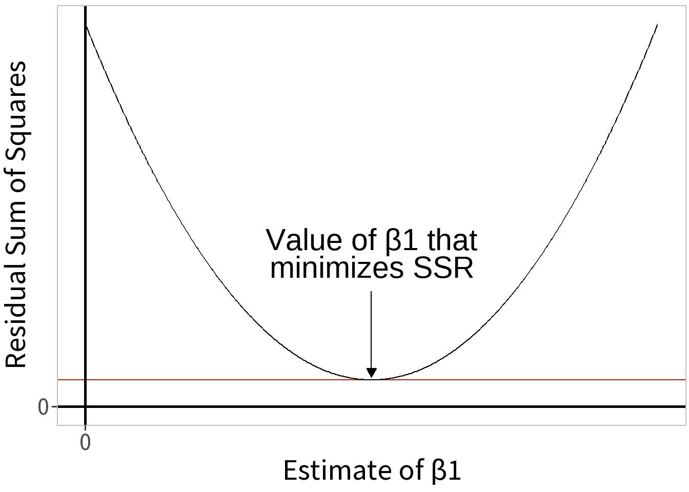
Ordinary Least Squares
A method for estimating the coefficients, \(\beta\), in a linear regression model by minimizing the Residual Sum of Squares, \(SS_{R}\).
\[SS_{R} = \sum_{i=1}^{n} (y_{i}-\hat{y}_i)^2\]
where \(\hat{y} \approx E[Y]\). To minimize this, we take its derivative with respect to \(\beta\) and set it equal to zero.
\[\frac{d\, SS_{R}}{d\, \beta} = 0\]
Simple estimators for coefficients:
Slope Ratio of covariance to variance \[\beta_{1} = \frac{cov(x, y)}{var(x)}\]
Intercept Conditional difference in means \[\beta_{0} = \bar{y} - \beta_1 \bar{x}\]
If \(\beta_{1} = 0\), then \(\beta_{0} = \bar{y}\).
🚗 Cars Model, again
Slope
\[\hat\beta_{1} = \frac{cov(x,y)}{var(x)} = \frac{10.426}{5.3847} = 1.9362\]
Intercept
\[ \begin{align} \hat\beta_{0} &= \bar{y} - \hat\beta_{1}\bar{x} \\[6pt] &= 10.54 - 1.9362 * 6.4821 \\[6pt] &= -2.0107 \end{align} \]