Lecture 03: Statistical Inference
1/24/23
Why statistics?


We want to understand something about a population.
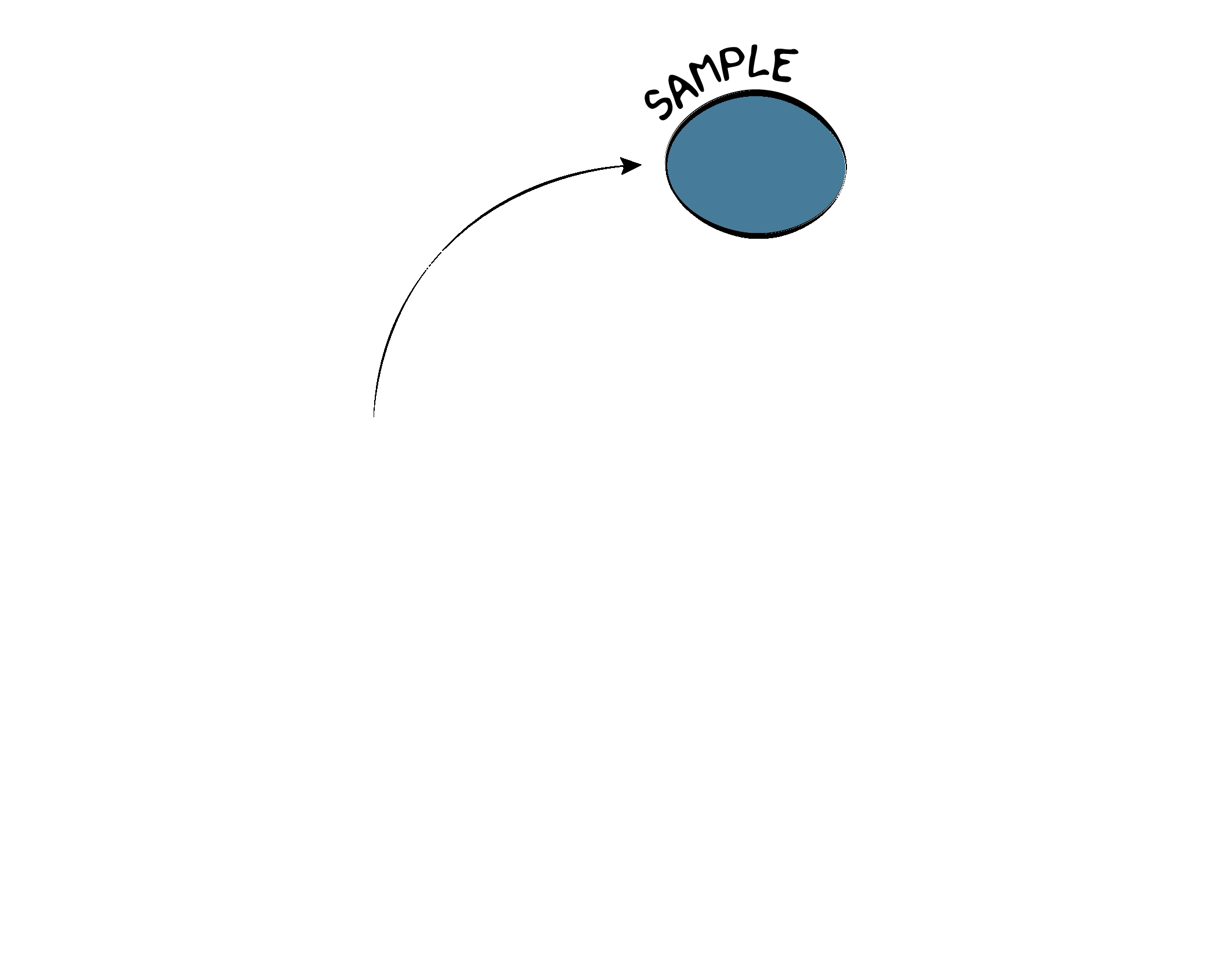
We can never observe the entire population, so we draw a sample.
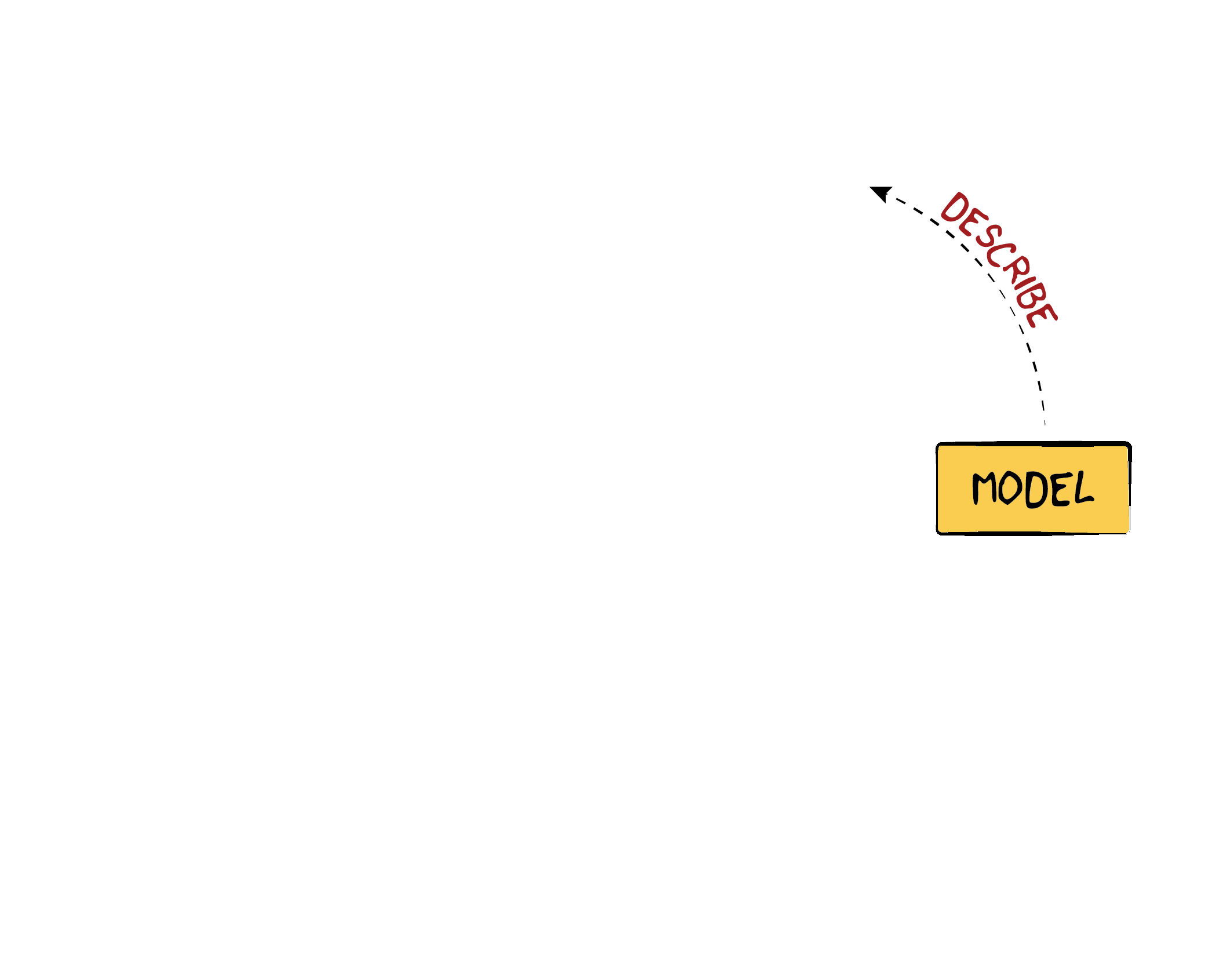
We then use a model to describe the sample.
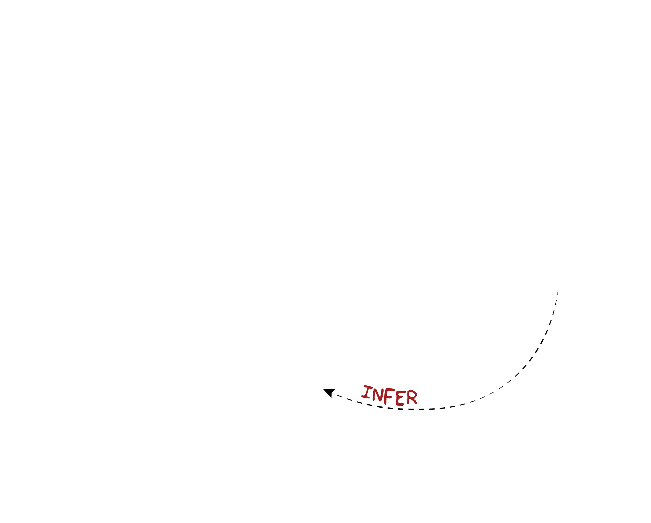
By comparing that model to a null model, we can infer something about the population.
Here, we’re going to focus on statistical inference.
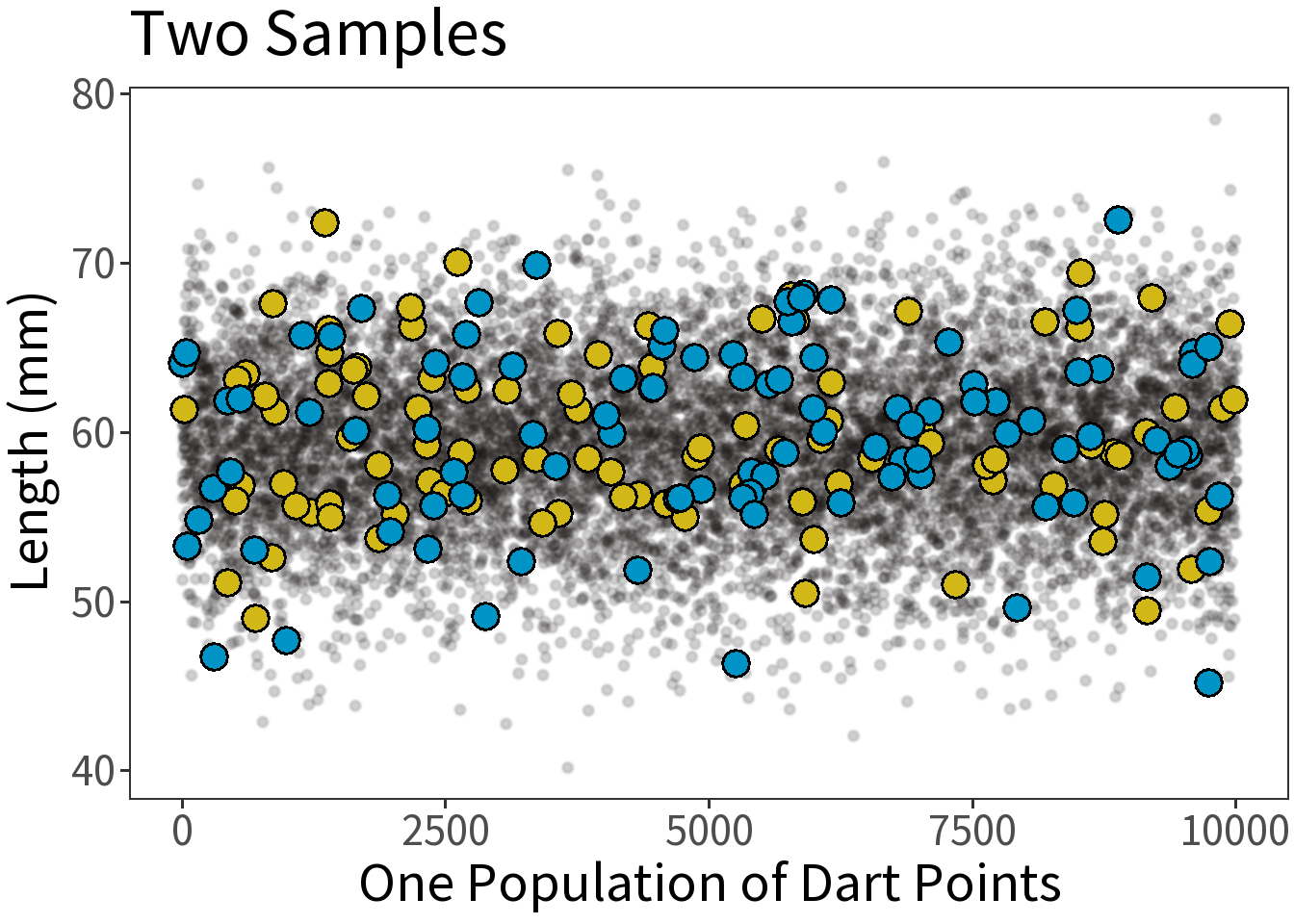
Simple Example
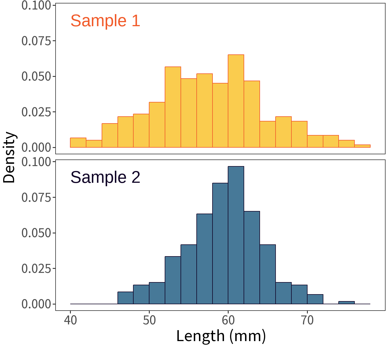
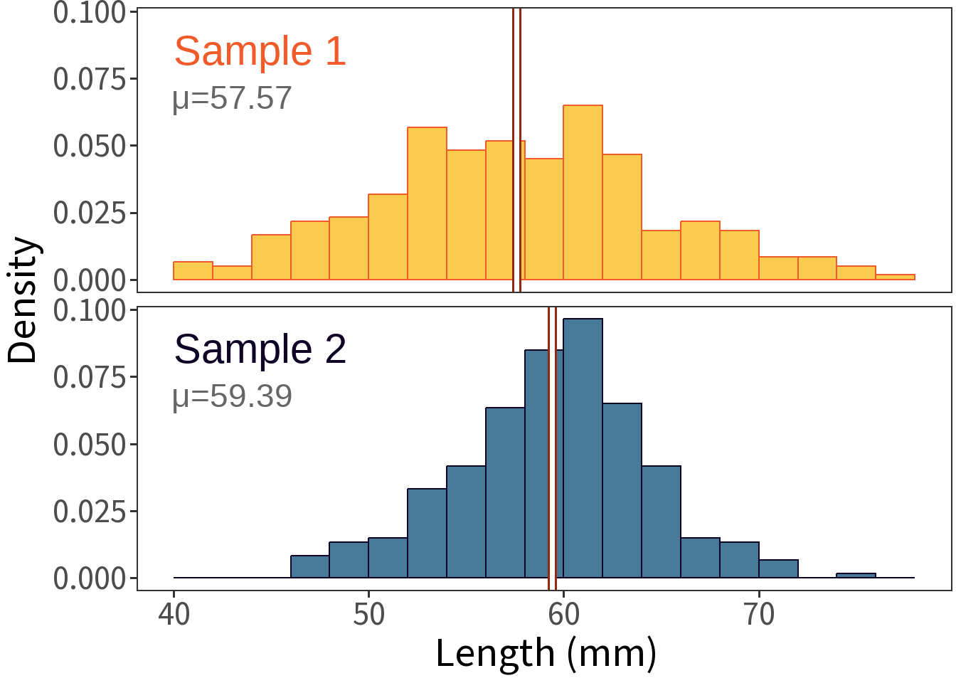
Two samples of length (mm, n=300).
Question: Are these samples of the same type? The same population?
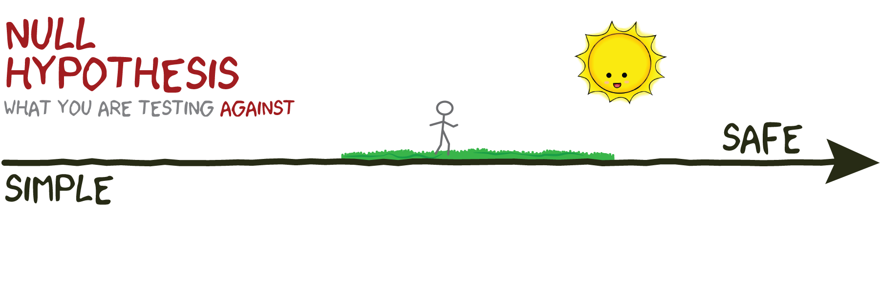
Hypotheses
The two models represent our hypotheses.
Testing Method
Procedure:
- Take sample(s).
- Calculate test statistic.
- Compare to test probability distribution.
- Get p-value.
- Compare to critical value.
- Accept (or reject) null hypothesis.
Average of differences
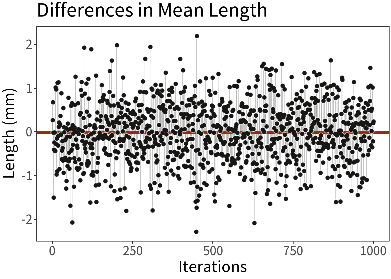
Suppose we take two samples from the same population, calculate the difference in their means, and repeat this 1,000 times.
Question: What will the average difference be between the sample means?
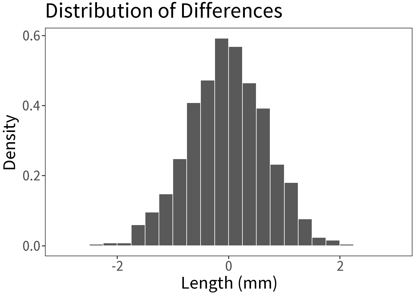
Probability of differences
If we convert these differences into a probability distribution, we can estimate the probability of any given difference.
The p-value represents how likely it is that the difference we see arises by chance.
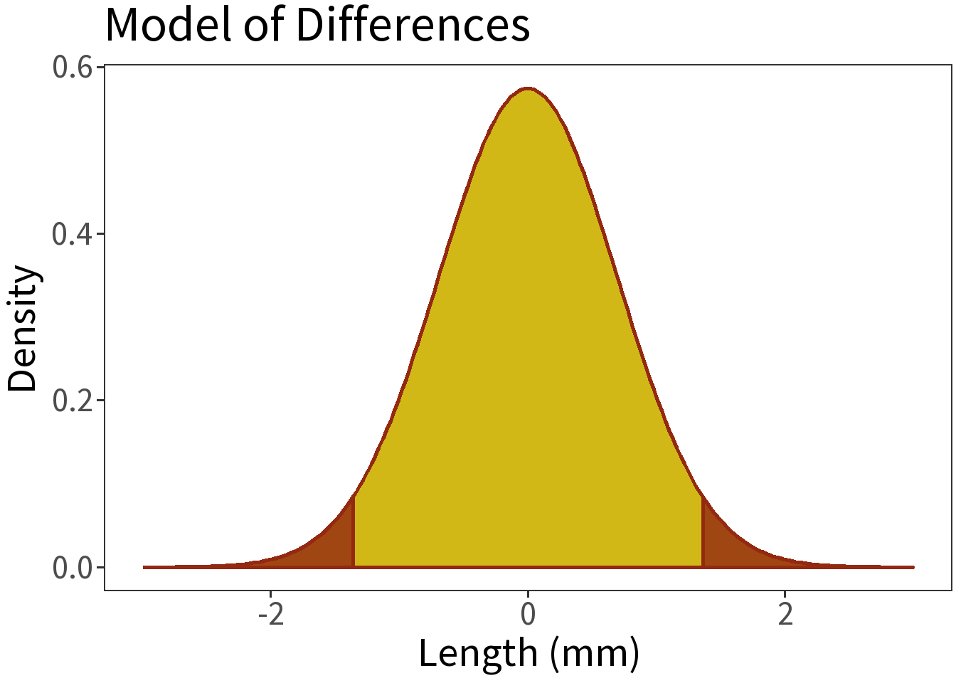
Model of Differences
In classical statistics, we use a model of that distribution to estimate the probability of a given difference. Here we are using \(N(0,\) 0.69\()\), where the probability of getting a difference \(\pm\) 1 mm (\(\pm2s\)) or greater is 0.05.

Rejecting the Null Hypothesis
Question: How do we decide?
Define a critical limit (\(\alpha\))
- Must be determined prior to the test!
- If \(p < \alpha\), reject. ← THIS IS THE RULE!
- Generally, \(\alpha = 0.05\)
Why the critical limit?
Because we might be wrong! But what kind of wrong?
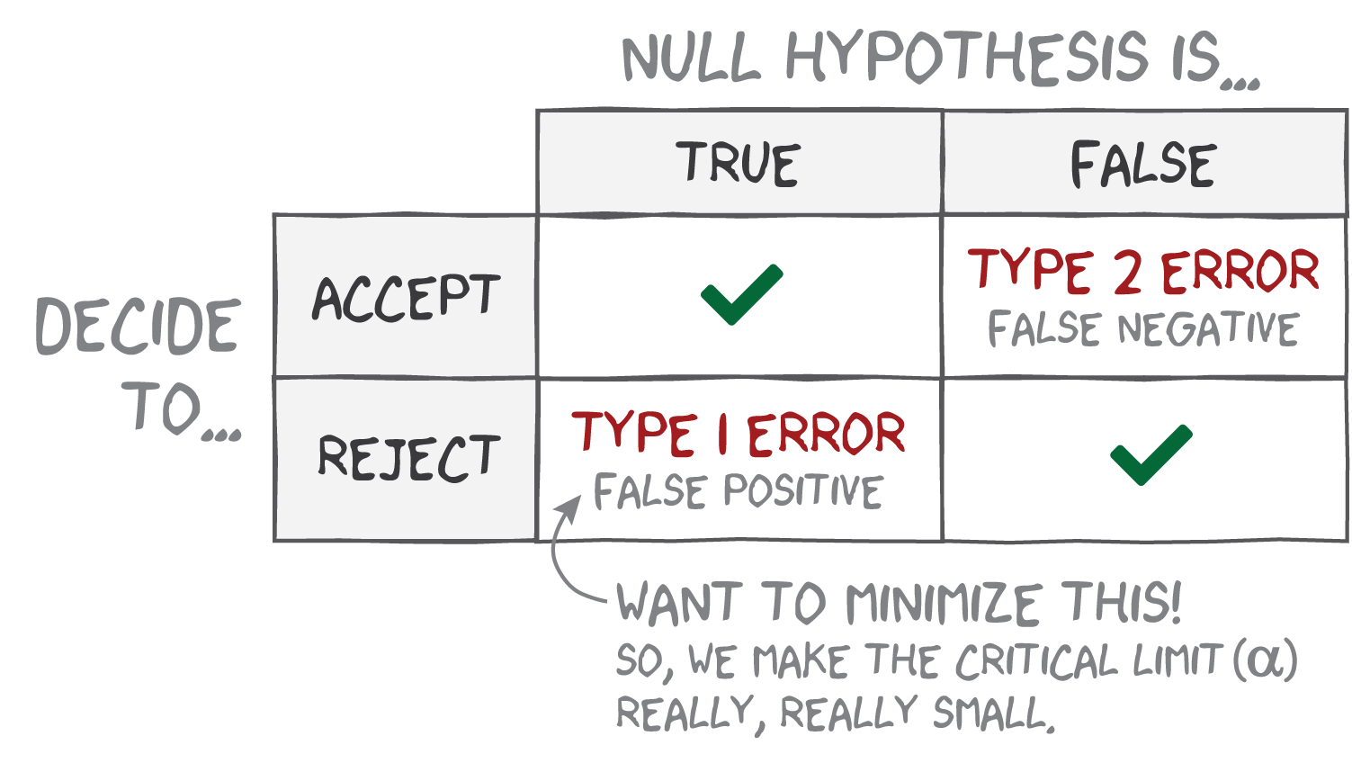
With \(\alpha=0.05\), we are saying, “If we run this test 100 times, only 5 of those tests should result in a Type 1 Error.”
Student’s t-test
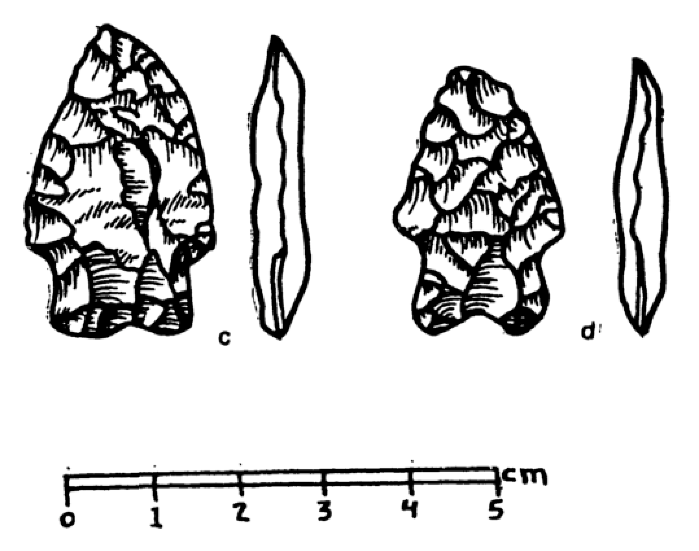
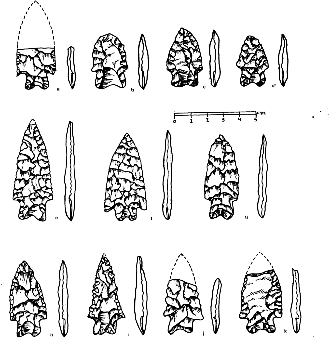
We have two samples of projectile points, each consisting of 300 measurements of length (mm).
Question: Are these samples of the same point type? The same population?
The null hypothesis:
\(H_0: \mu_1 = \mu_2\)
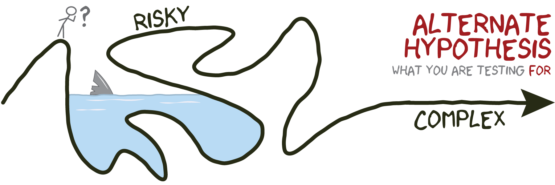
The alternate hypothesis:
\(H_1: \mu_1 \neq \mu_2\)
This is a two-sided t-test as the difference can be positive or negative.
Question: Is this difference (-1.82) big enough to reject the null?
A t-statistic standardizes the difference in means using the standard error of the sample mean.
\[t = \frac{\bar{x}_1 - \bar{x}_2}{s_{\bar{x}}}\]
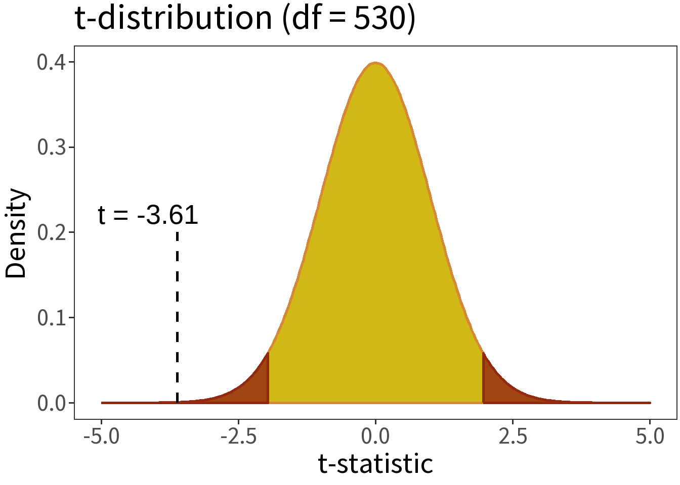
For our samples, \(t =\) -3.61. This is a model of our data!
Question: How probable is this estimate?
We can answer this by comparing the t-statistic to the t-distribution.
But first, we need to evaluate how complex the t-statistic is. We do this by estimating the degrees of freedom, or the number of values that are free to vary after calculating a statistic. In this case, we have two samples with 300 observations each, hence:
df = 530
Crucially, this affects the shape of the t-distribution and, thus, determines the location of the critical value we use to evaluate the null hypothesis.
Summary:
- \(\alpha = 0.05\)
- \(H_{0}: \mu_1 = \mu_2\)
- \(p =\) 0.0003
Translation: the null hypothesis is really, really unlikely. So, there must be some difference in the mean!
ANOVA
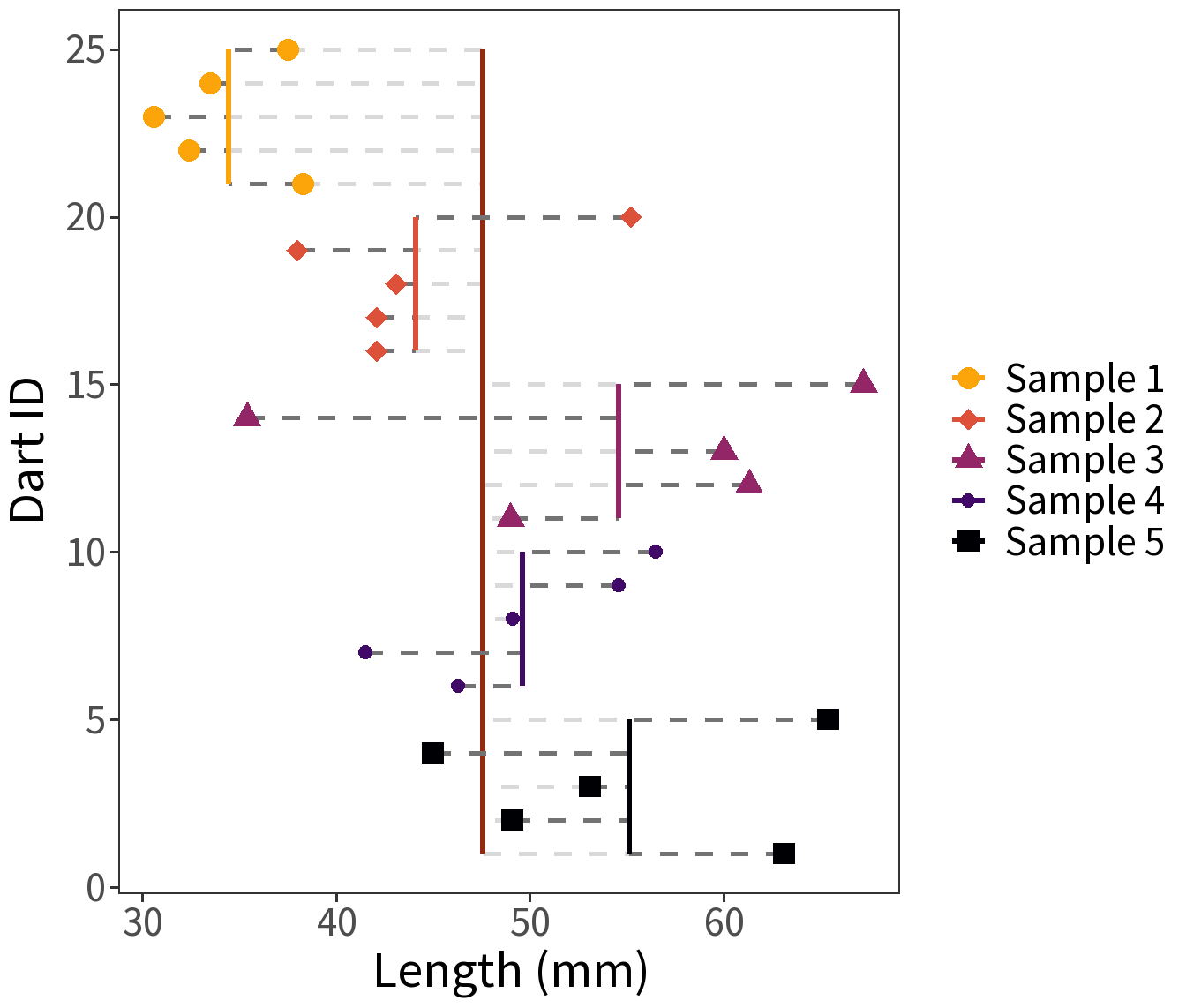
We have five samples of points, each consisting of 100 measurements of length (mm).
Question: Are these samples of the same point type? The same population?
Analysis of Variance (ANOVA) is like a t-test but for more than two samples.
The null hypothesis:
\(H_0:\) no difference between groups
The alternate hypothesis:
\(H_1:\) at least one group is different
Variance Decomposition. When group membership is known, the contribution of any value \(x_{ij}\) to the variance can be split into two parts:
\[(x_{ij} - \bar{x}) = (\bar{x}_{j} - \bar{x}) + (x_{ij} - \bar{x}_{j})\]
where
- \(i\) is the \(i\)th observation,
- \(j\) is the \(j\)th group,
- \(\bar{x}\) is the between-group mean, and
- \(\bar{x_{j}}\) is the within-group mean (of group \(j\)).

Sum and square the differences for all \(n\) observation and \(m\) groups gives us:
\[SS_{T} = SS_{B} + SS_{W}\]
where
- \(SS_{T}\): Total Sum of Squares
- \(SS_{B}\): Between-group Sum of Squares
- \(SS_{W}\): Within-group Sum of Squares
Ratio of variances:
\[F = \frac{\text{between-group variance}}{\text{within-group variance}}\]
where
- Between-group variance = \(SS_{B}/df_{B}\) and \(df_{B}=m-1\).
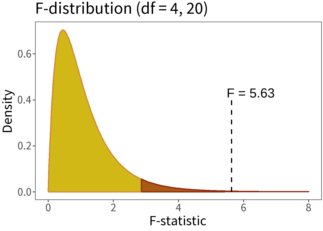
- Within-group variance = \(SS_{W}/df_{W}\) and \(df_{W}=m(n-1)\).
Question: Here, \(F=\) 5.63. How probable is this estimate?
We can answer this question by comparing the F-statistic to the F-distribution.
Summary:
- \(\alpha = 0.05\)
- \(H_{0}:\) no difference
- \(p=\) 0.003
Translation: the null hypothesis is really, really unlikely, so there must be some difference between groups!