Lecture 02: Probability as a Model
2/20/23
Why statistics?
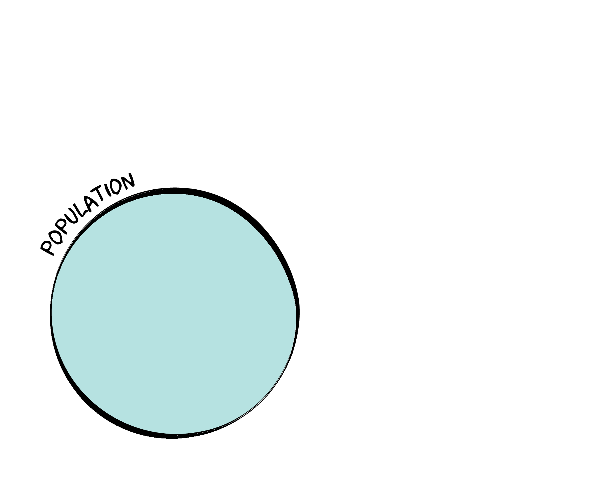

We want to understand something about a population.
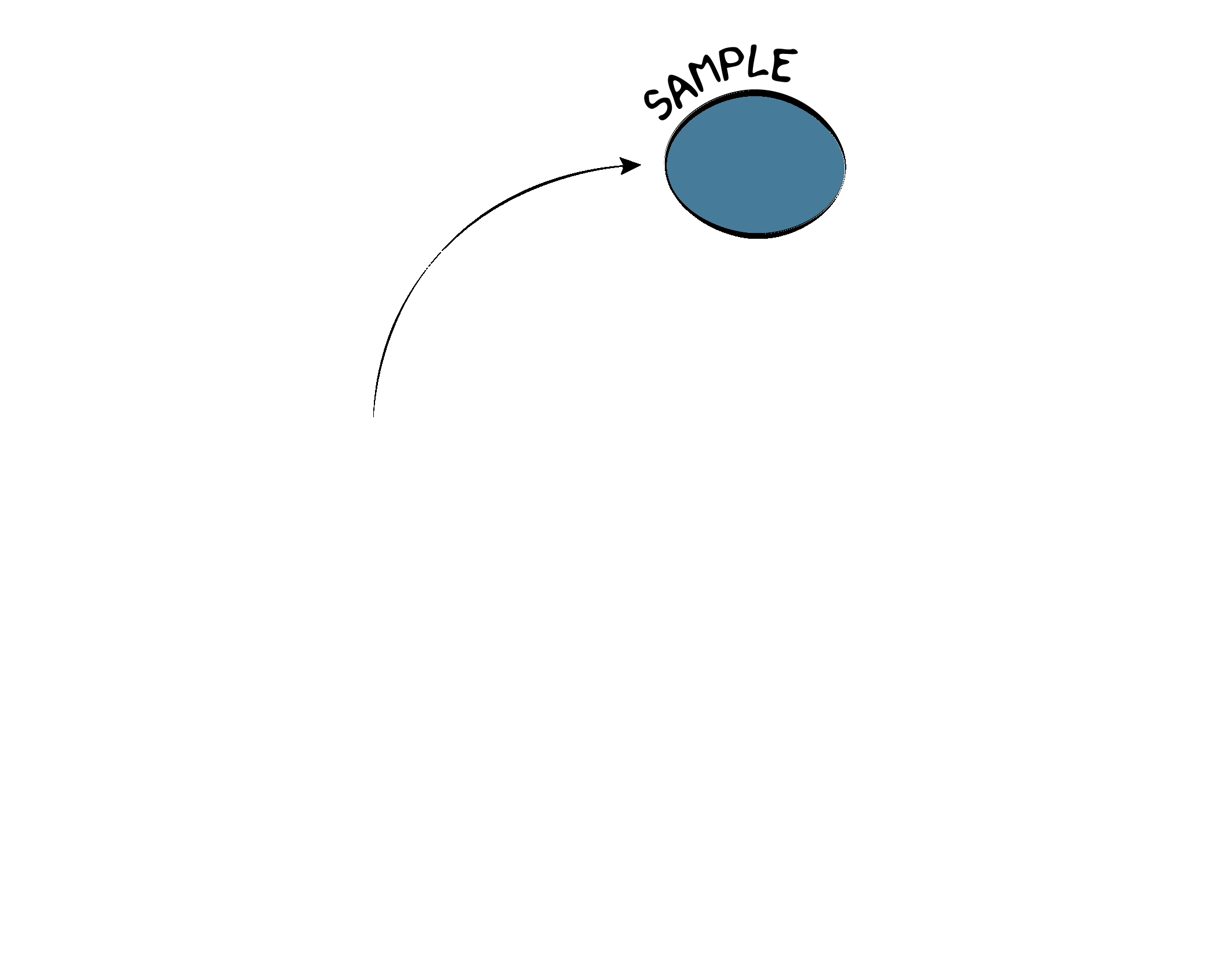
We can never observe the entire population, so we draw a sample.
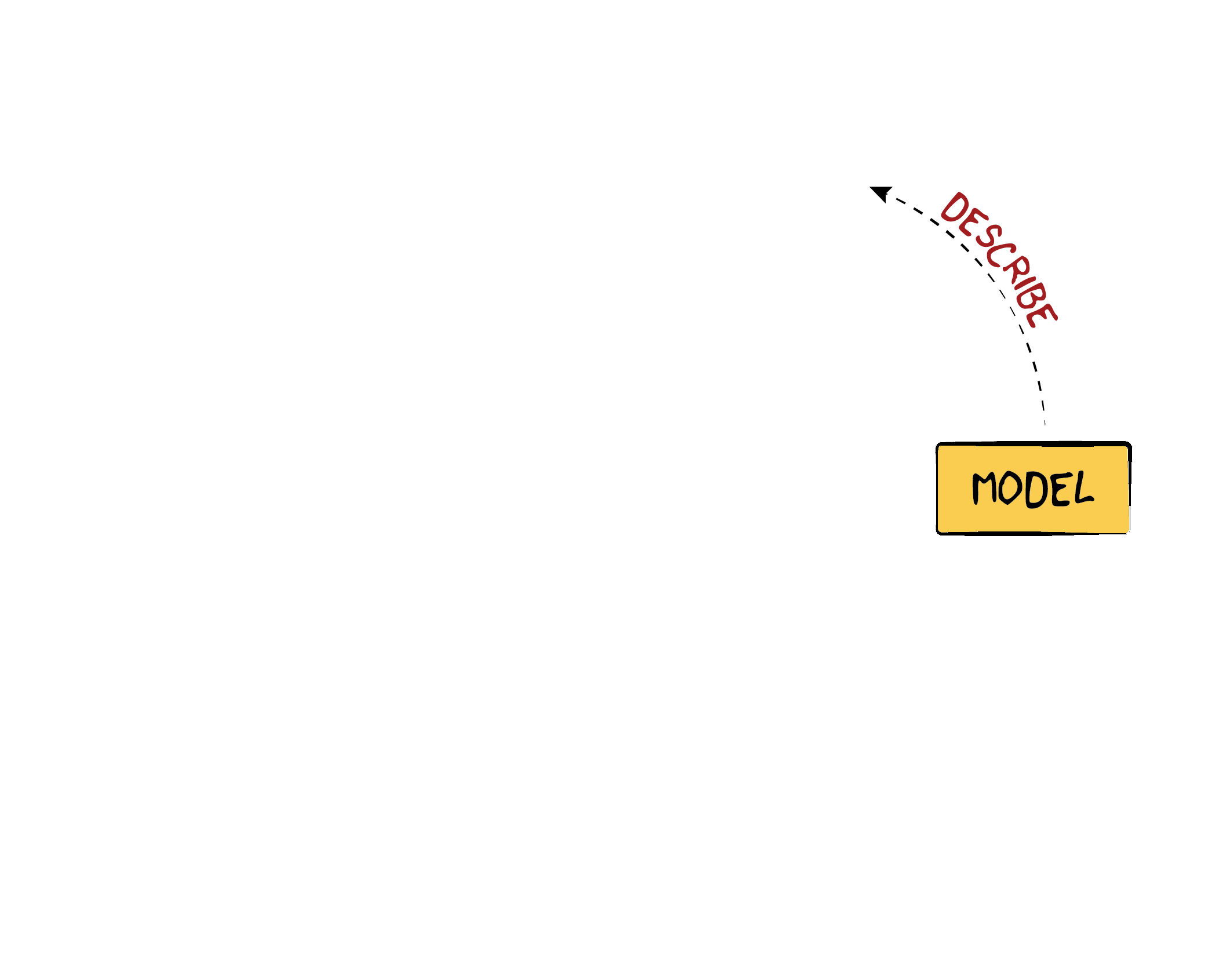
We then use a model to describe the sample.
By comparing that model to a null model, we can infer something about the population.
Here, we’re going to focus on statistical description, aka models.
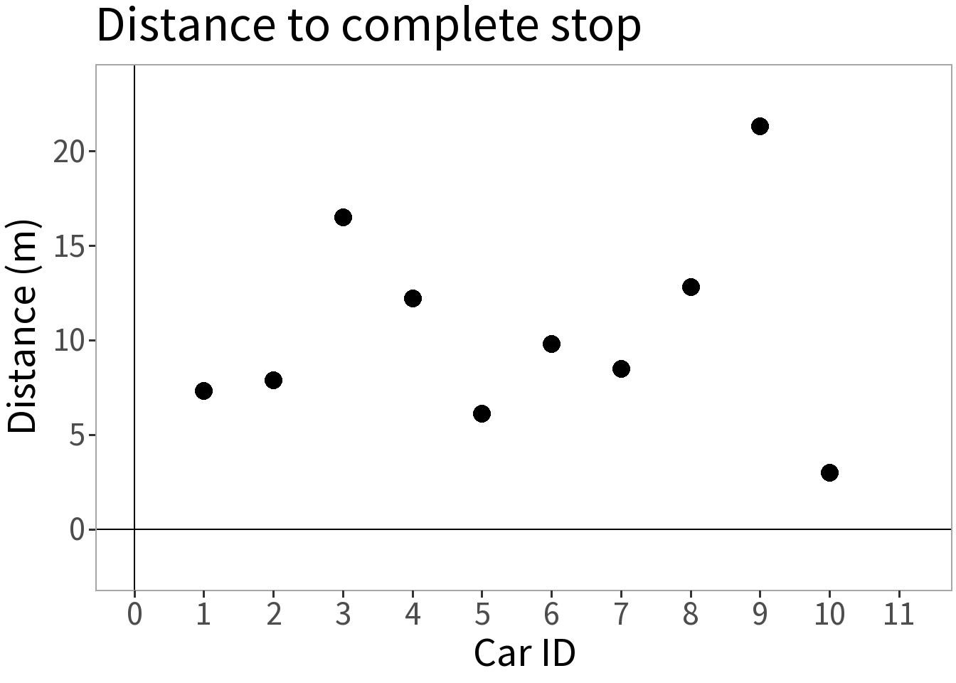
🧪 A simple experiment
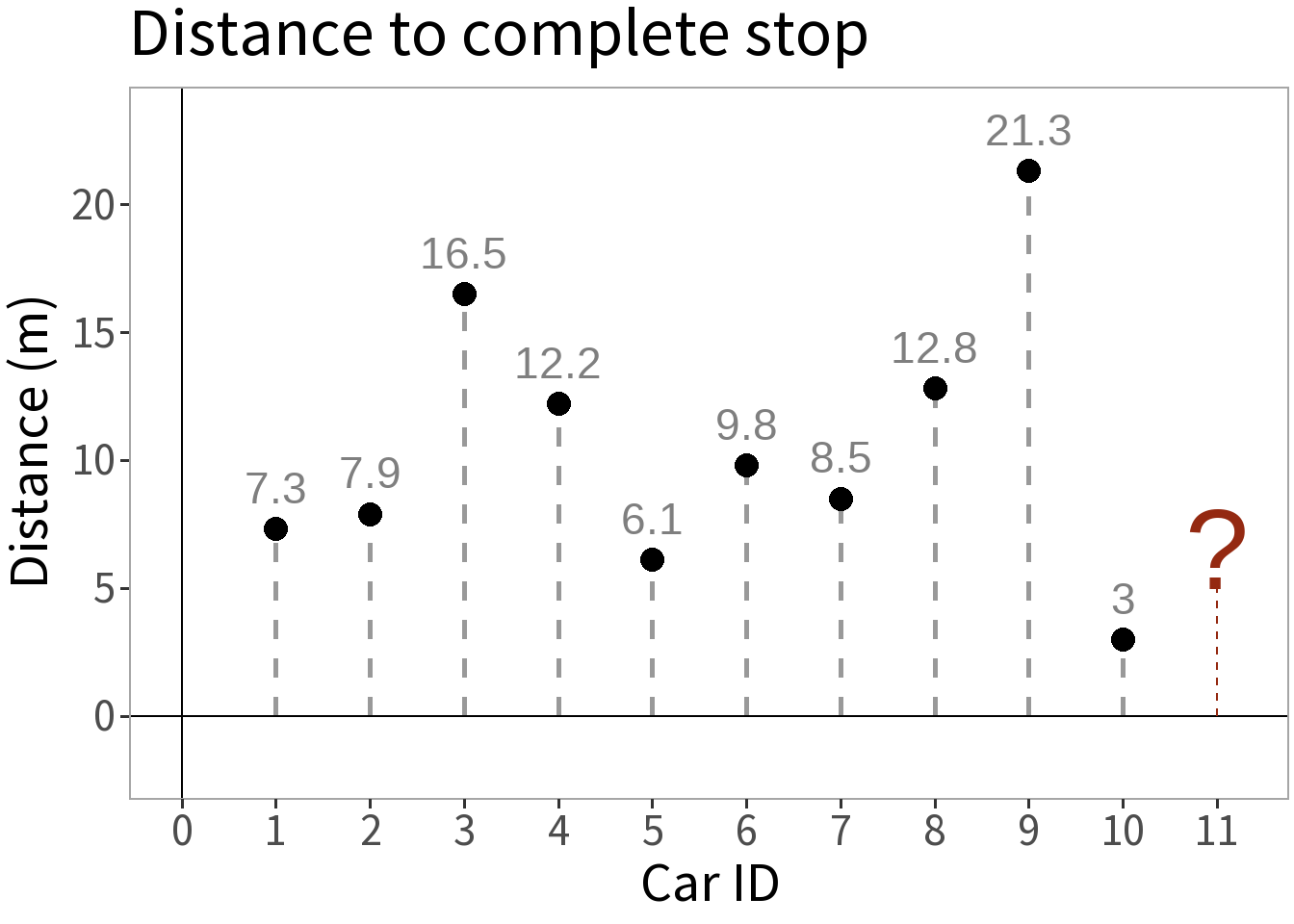
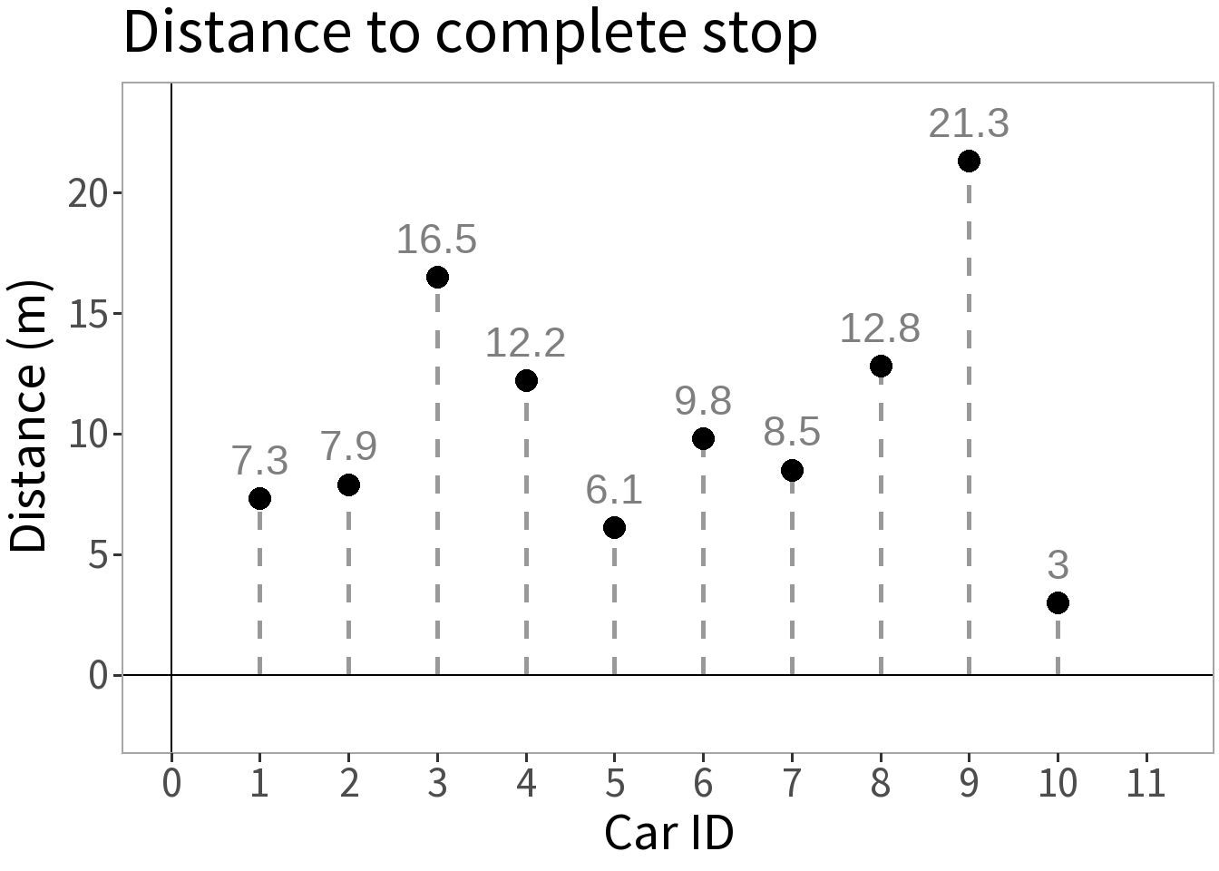
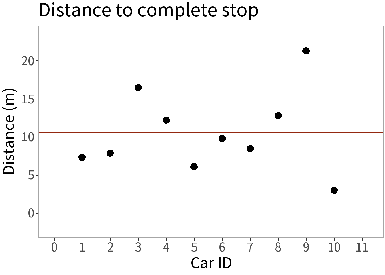
We take ten cars, send each down a track, have them brake at the same point, and measure the distance it takes them to stop.
Question: how far do you think it will take the next car to stop?
Question: what distance is the most probable?
But, how do we determine this?
Some terminology

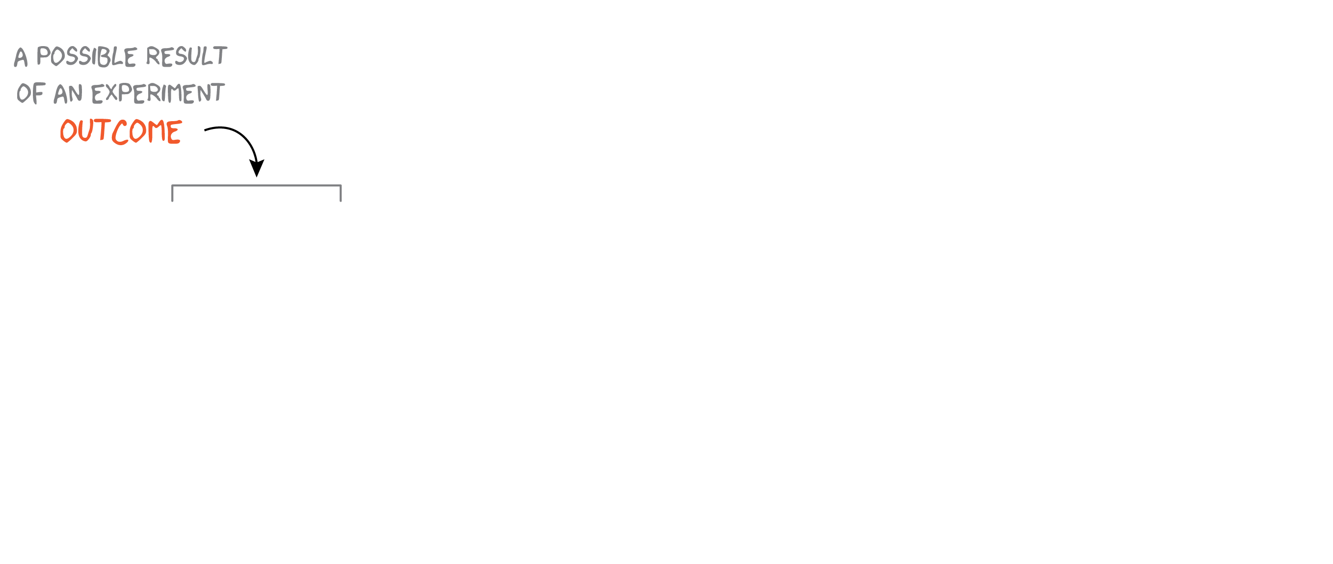
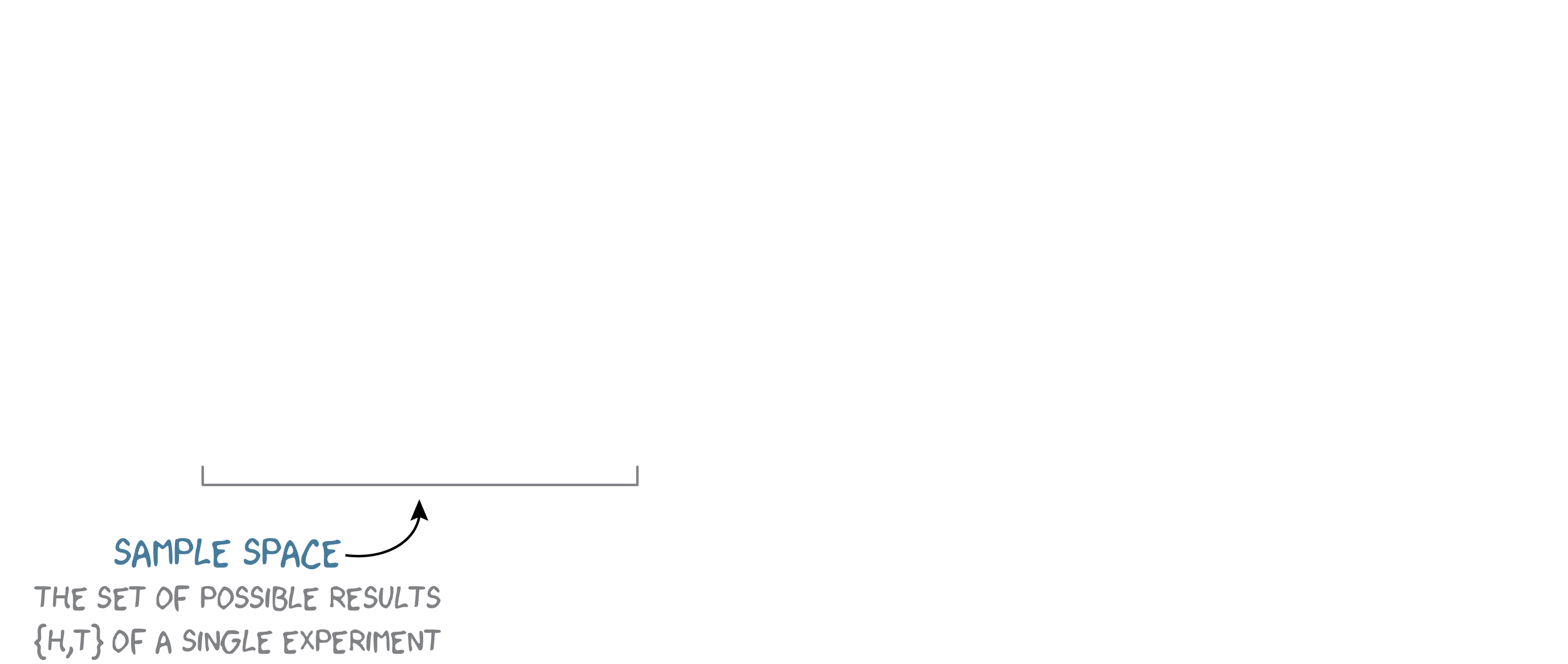
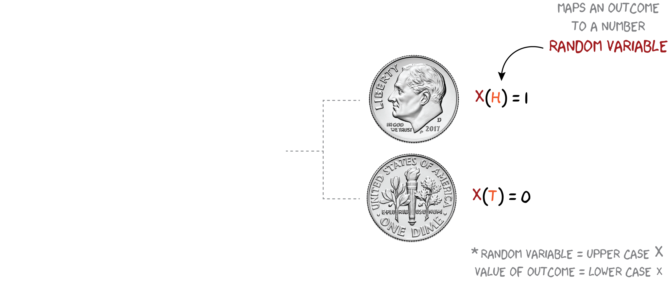
🎲 Probability
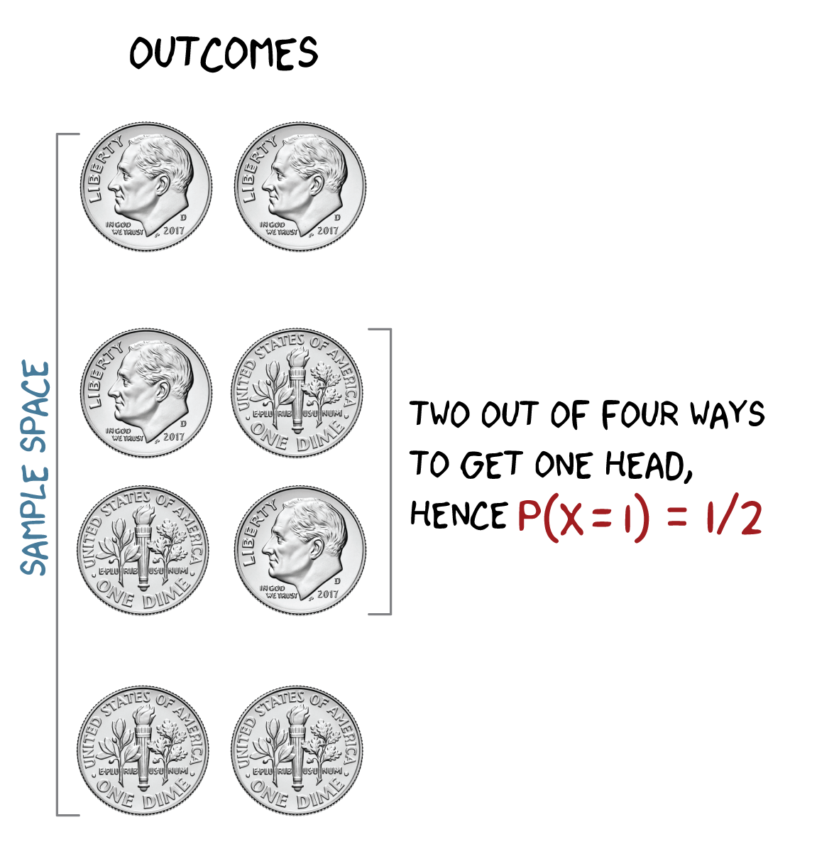
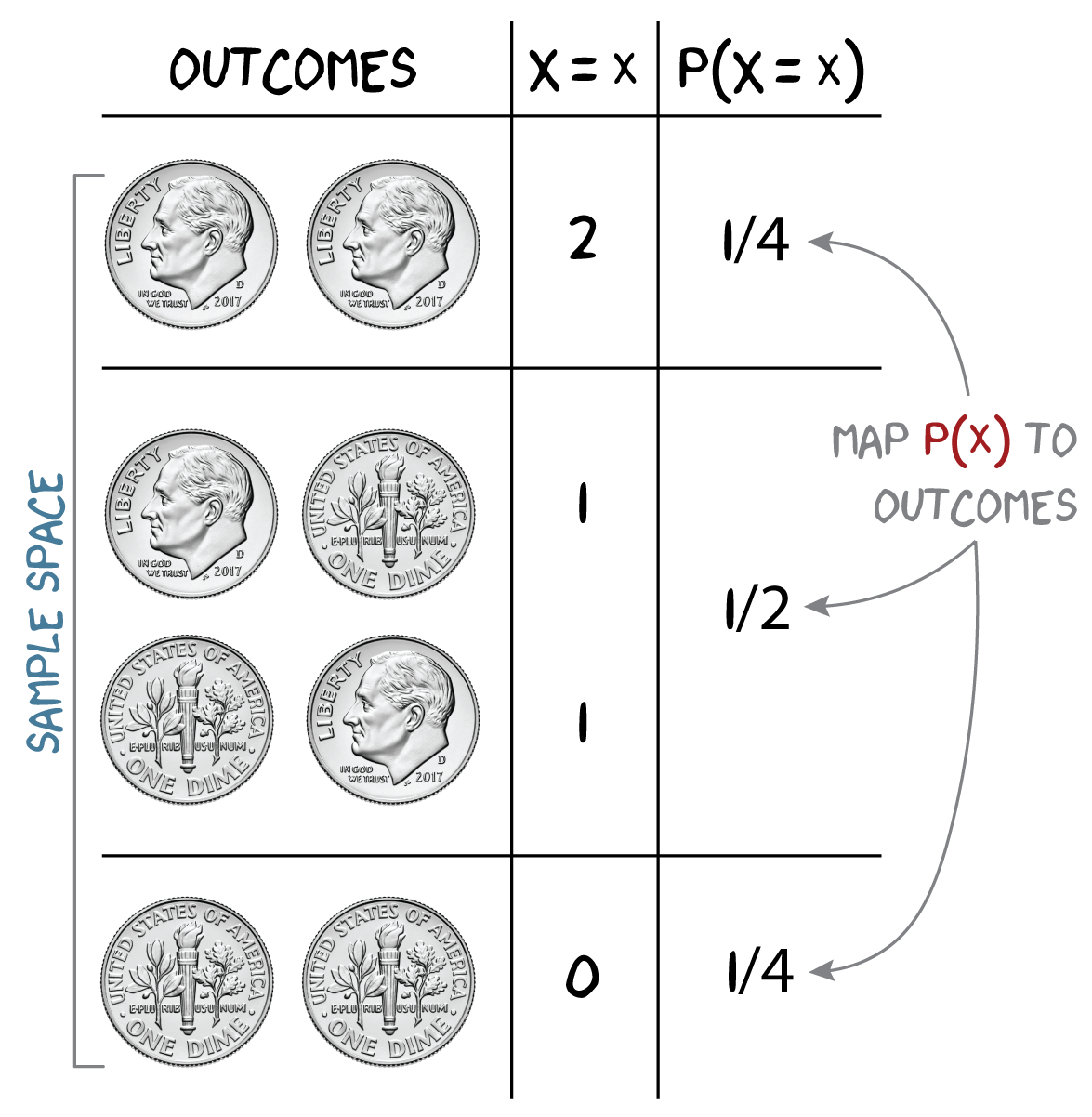
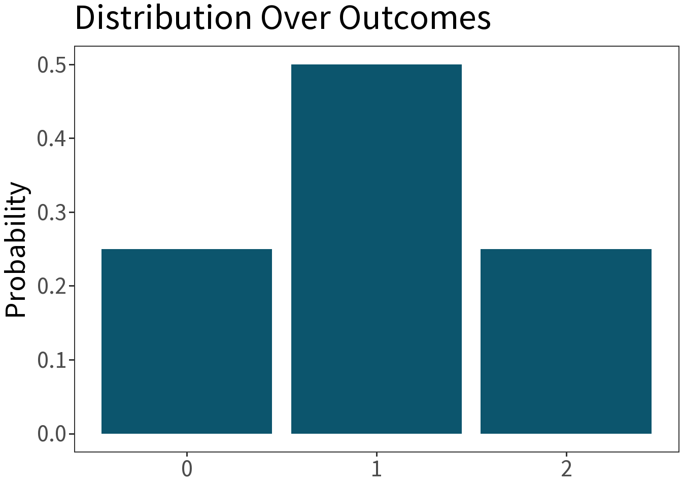
Let \(X\) be the number of heads in two tosses of a fair coin. What is the probability that \(X=1\)?
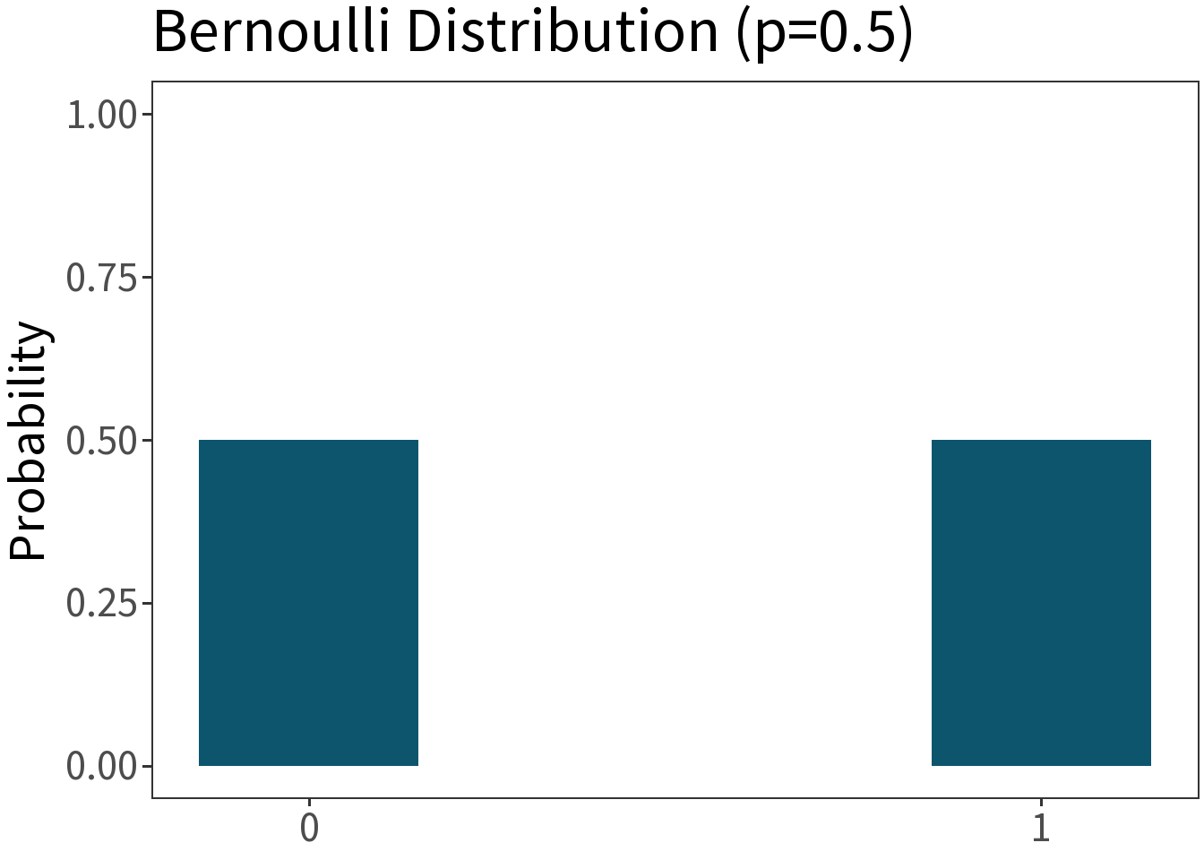
Bernoulli
Df. distribution of a binary random variable (“Bernoulli trial”) with two possible values, 1 (success) and 0 (failure), with \(p\) being the probability of success. E.g., a single coin flip.
\[f(x,p) = p^{x}(1-p)^{1-x}\]
Mean: \(p\)
Variance: \(p(1-p)\)
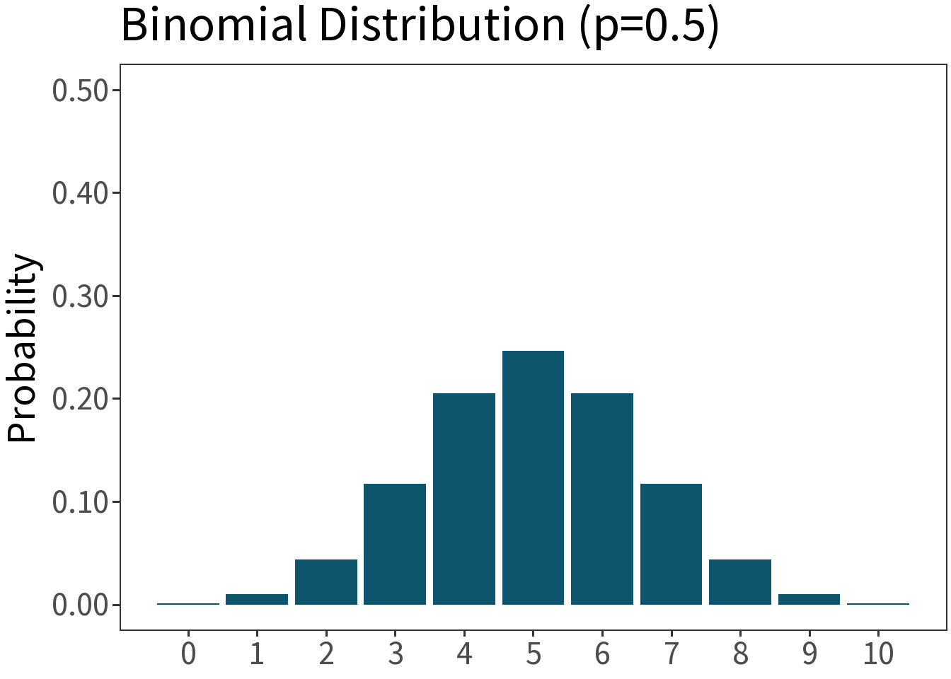
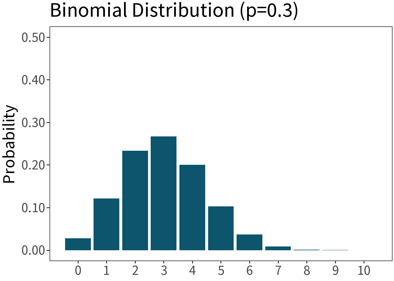
Binomial
Df. distribution of a random variable whose value is equal to the number of successes in \(n\) independent Bernoulli trials. E.g., number of heads in ten coin flips.
\[f(x,p,n) = \binom{n}{x}p^{x}(1-p)^{1-x}\]
Mean: \(np\)
Variance: \(np(1-p)\)
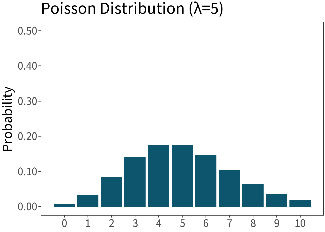
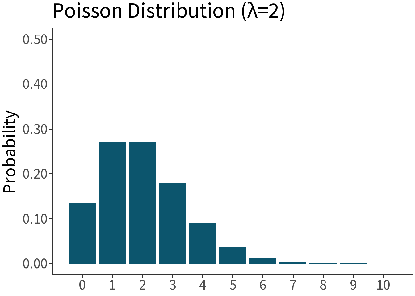
Poisson
Df. distribution of a random variable whose value is equal to the number of events occurring in a fixed interval of time or space. E.g., number of orcs passing through the Black Gates in an hour.
\[f(x,\lambda) = \frac{\lambda^{x}e^{-\lambda}}{x!}\]
Mean: \(\lambda\)
Variance: \(\lambda\)
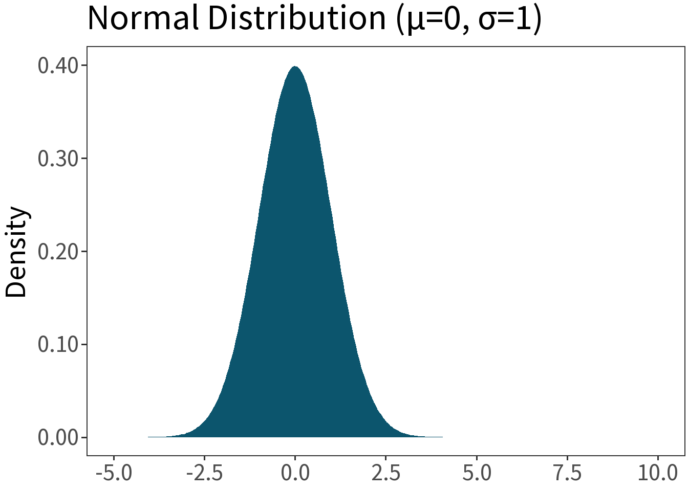
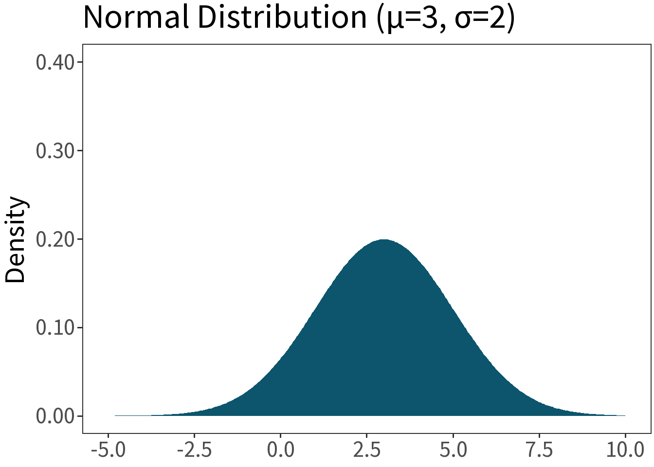
Normal (Gaussian)
Df. distribution of a continuous random variable that is symmetric from positive to negative infinity. E.g., the height of actors who auditioned for the role of Aragorn.
\[f(x,\mu,\sigma) = \frac{1}{\sqrt{2\pi\sigma^2}}\;exp\left[-\frac{1}{2}\left(\frac{x-\mu}{\sigma}\right)^2\right]\]
Mean: \(\mu\)
Variance: \(\sigma^2\)
🚗 Cars Model
Let’s use the Normal distribution to describe the cars data.
- \(Y\) is stopping distance for population
- \(Y\) is normally distributed, \(Y \sim N(\mu, \sigma)\)
- Experiment is a random sample of size \(n\) from \(Y\) with \(y_1, y_2, ..., y_n\) observations.
- Sample statistics (\(\bar{y}, s\)) approximate population parameters (\(\mu, \sigma\)).
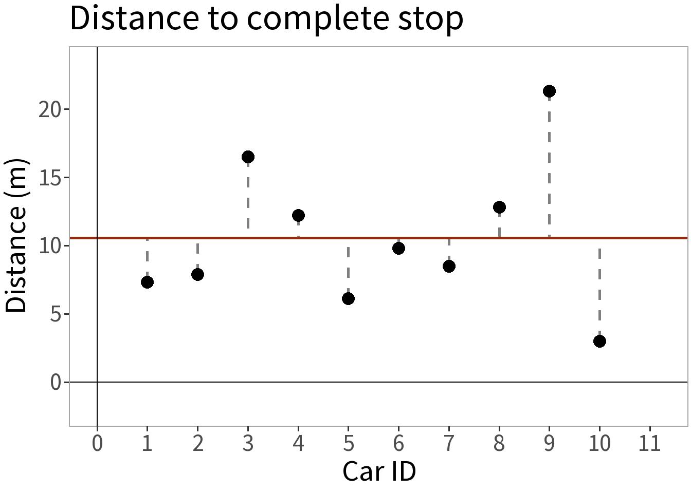
Sample statistics:
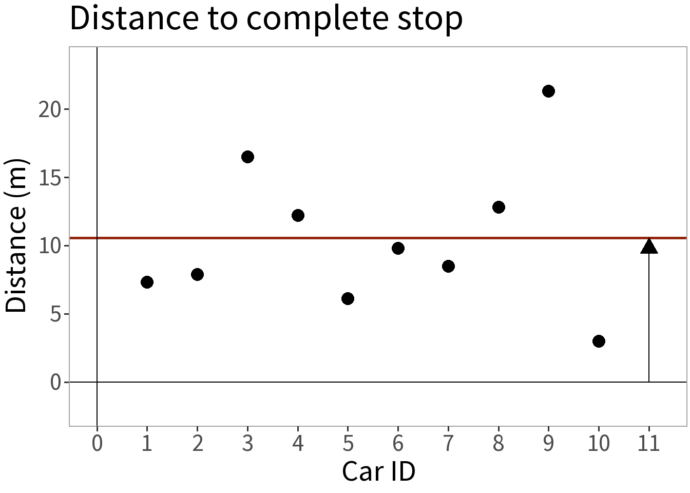
- Mean (\(\bar{y}\)) = 10.54 m
Sample statistics:
- Mean (\(\bar{y}\)) = 10.54 m
This is our approximate expectation
- \(E[Y] = \mu \approx \bar{y}\)
Sample statistics:
- Mean (\(\bar{y}\)) = 10.54 m
But, there’s error, \(\epsilon\), in this estimate.
- \(\epsilon_i = y_i - \bar{y}\)
Sample statistics:
- Mean (\(\bar{y}\)) = 10.54 m
The average squared error is the variance:
- \(s^2 = \frac{1}{n-1}\sum \epsilon_{i}^{2}\)
Sample statistics:
- Mean (\(\bar{y}\)) = 10.54 m
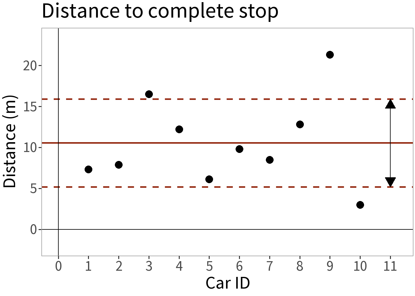
- S.D. (\(s\)) = 5.353 m
This is our uncertainty, how big we think any given error will be.
Sample statistics:
- Mean (\(\bar{y}\)) = 10.54 m
- S.D. (\(s\)) = 5.353 m
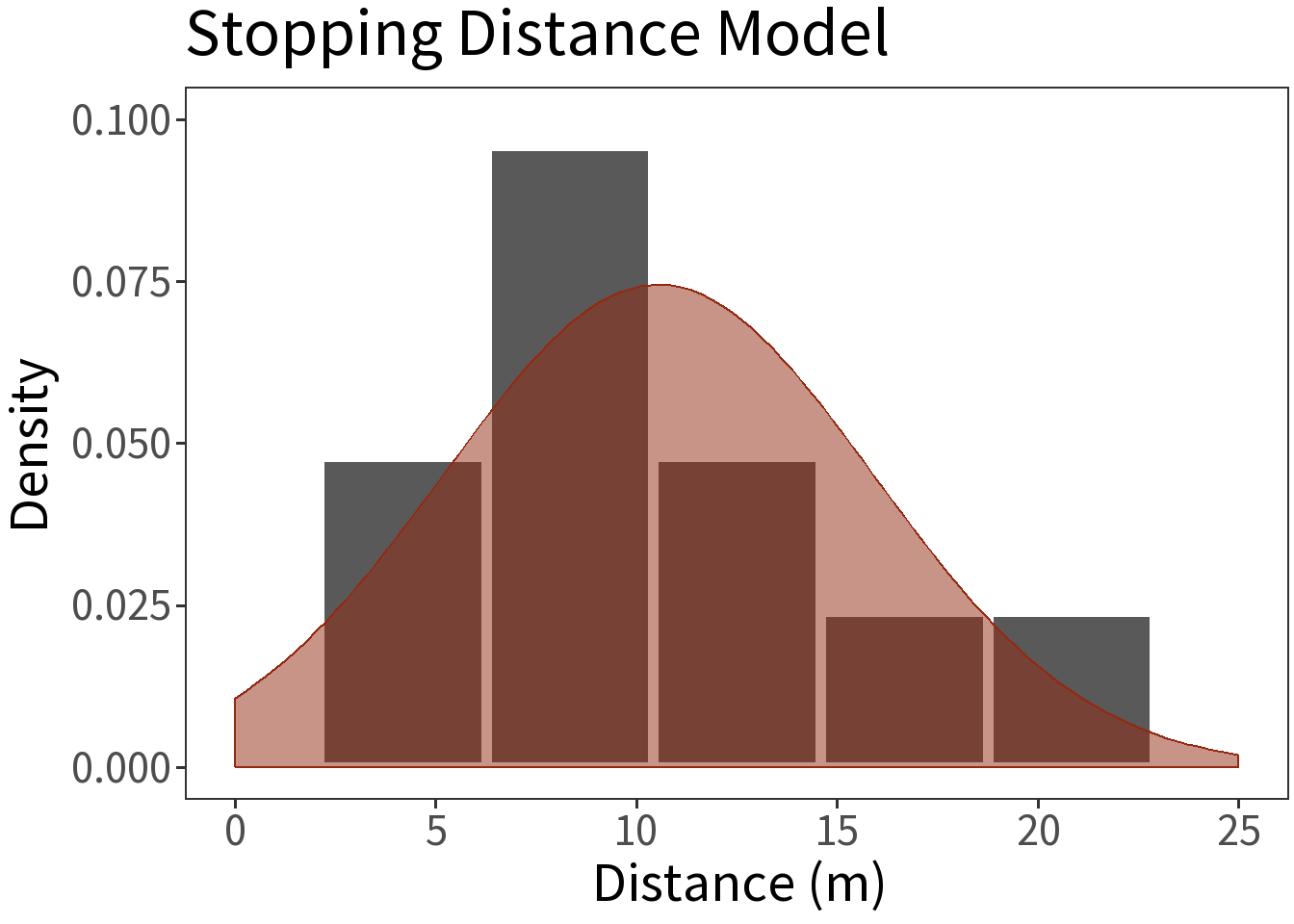
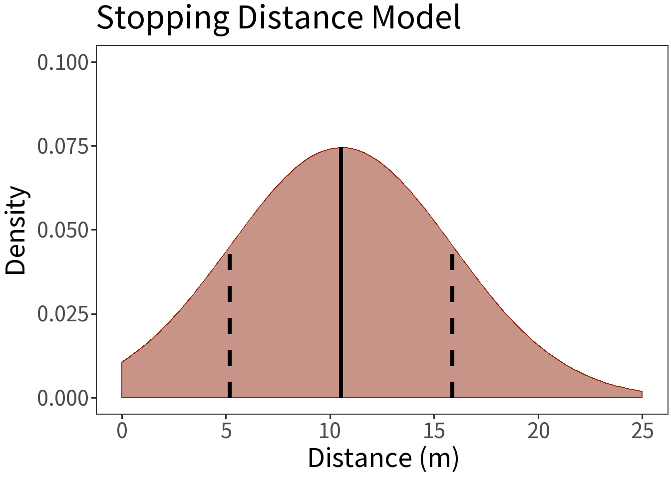
So, here is our probability model.
\[Y \sim N(\bar{y}, s)\] This is only an estimate of \(N(\mu, \sigma)\)!
Sample statistics:
- Mean (\(\bar{y}\)) = 10.54 m
- S.D. (\(s\)) = 5.353 m
With it, we can say, for example, that the probability that a random draw from this distribution falls within one standard deviation (dashed lines) of the mean (solid line) is 68.3%.


A Simple Formula
This gives us a simple formula
\[y_i = \bar{y} + \epsilon_i\] where
- \(y_i\): stopping distance for car \(i\), data
- \(\bar{y} \approx E[Y]\): expectation, predictable
- \(\epsilon_i\): error, unpredictable
This gives us a simple formula
\[y_i = \bar{y} + \epsilon_i\]
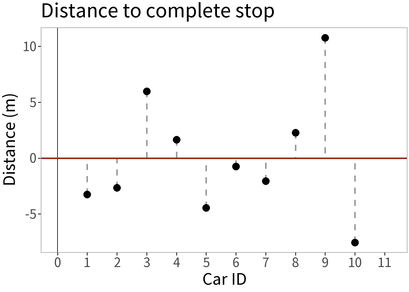
If we subtract the mean, we have a model of the errors centered on zero:
\[\epsilon_i = 0 + (y_i - \bar{y})\]
This gives us a simple formula
\[y_i = \bar{y} + \epsilon_i\]
If we subtract the mean, we have a model of the errors centered on zero:
\[\epsilon_i = 0 + (y_i - \bar{y})\]
This means we can construct a probability model of the errors centered on zero.
Probability Model of Errors
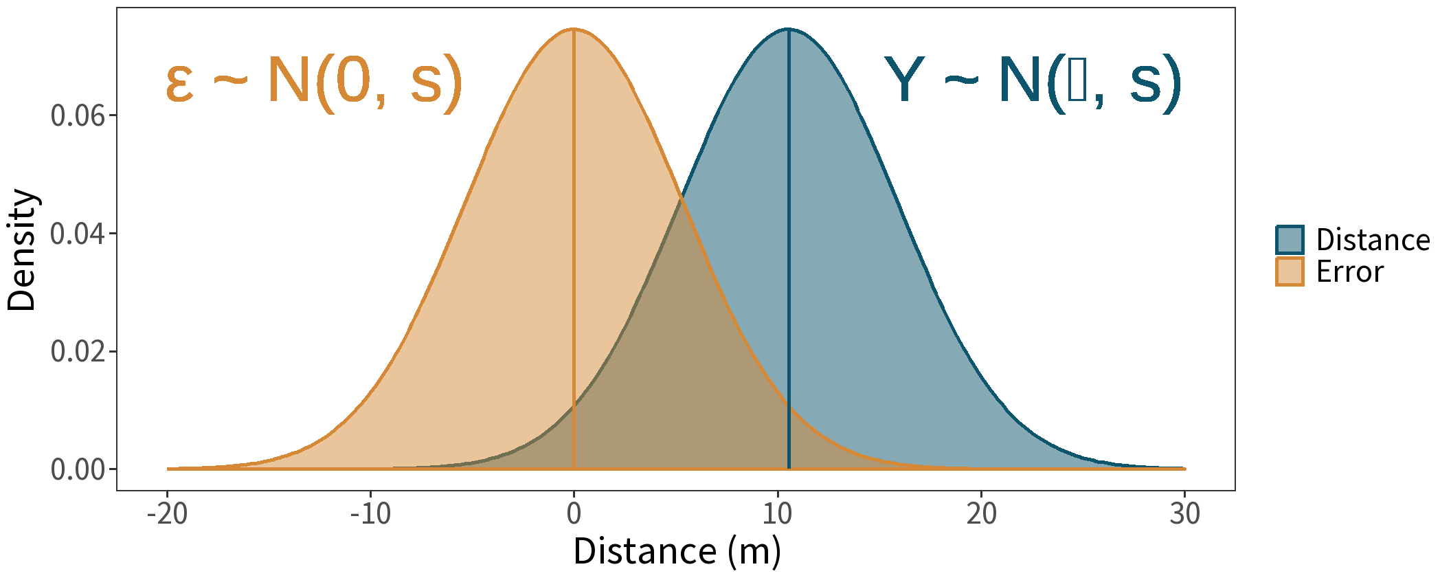
Note that the mean changes, but the variance stays the same.