Lab 06: Working with Tables

A review and a deep dive into working with rectangular data in R.

Outline

Objectives

This lab will guide you through the process of

• constructing data.frames and tibbles
• working with the pipe
• working with columns (variables) in a table
• working with rows (observations) in a table
• working with grouped data in a table

R Packages

• archdata
• palmerpenguins
• dplyr

library(archdata)
library(palmerpenguins)
library(dplyr)

Data

• penguins
  • Includes measurements for penguin species, island in Palmer Archipelago, size (flipper length, body mass, bill dimensions), and sex.
  • package: palmerpenguins
  • reference: https://allisonhorst.github.io/palmerpenguins/reference/penguins.html
• DartPoints
  • Includes measurements of 91 Archaic dart points recovered during surface surveys at Fort Hood, Texas.
  • package: archdata
  • reference: https://cran.r-project.org/web/packages/archdata/archdata.pdf

Tables

Figure 1: Elements of a Data Frame.

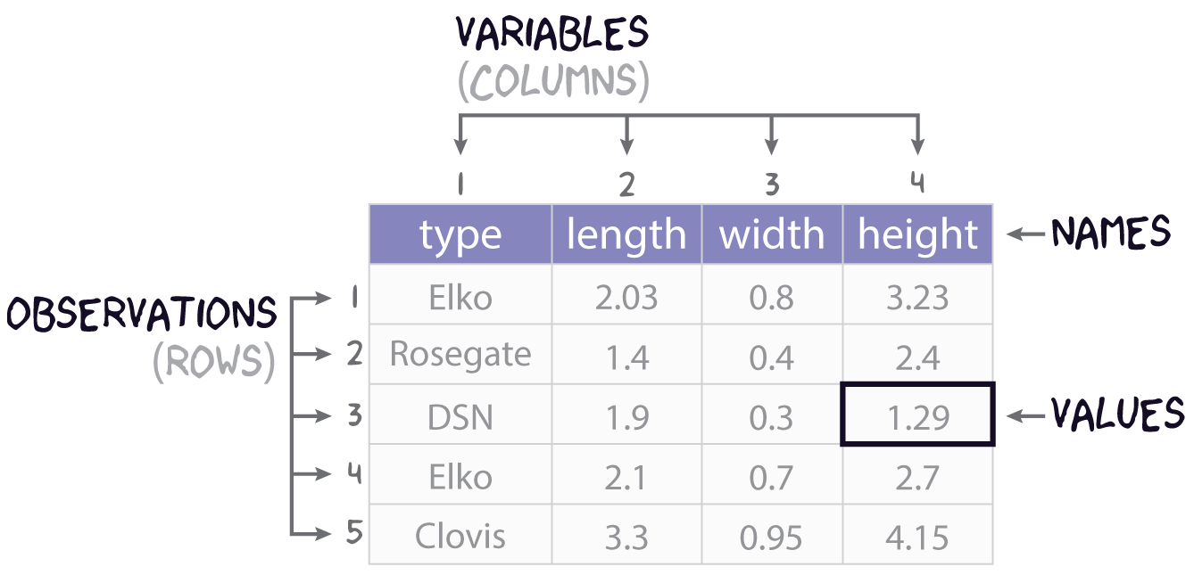
Consider this research scenario: you have a museum collection of projectile points that you want to use for an analysis, maybe you want to know whether East Gate and Rose Spring points are actually the same type of point, commonly referred to using the portmanteau Rosegate. Following tradition, you think maybe it’s the size and shape that will you help finally put this old question to rest, so for each individual point, you set about measuring its length, width, and height.

In this course, we’ll refer to each individual measure that you make as a value, each set of such measures for an individual point we will call (somewhat awkwardly) an observation, and each individual type of measurement will be a variable. It is almost certainly the case that you will be collecting this data and storing it in something like a spreadsheet or table, like that shown in Figure 1. You will sometimes hear data scientists refer to data stored in this way as rectangular data. All they mean by that is that the data come as collections of values organized into rows and columns. Crucially, all the columns must have the same length, so you can describe the data as having dimensions, specifically length (the number of observations or rows) and width (the number of variables or columns).

Creating tables

In R, tabular datasets are known as data frames. To create a data frame, we use the eponymous data.frame() function. Here, for example, is how we would create the table in Figure 1 above:

projectiles_df <- data.frame(
  type = c("Elko", "Rosegate", "DSN", "Elko", "Clovis"),
  length = c(2.03, 1.4, 1.9, 2.1, 3.3),
  width = c(0.8, 0.4, 0.3, 0.7, 0.95),
  height = c(3.23, 2.4, 1.29, 2.7, 4.15)
)

projectiles_df

      type length width height
1     Elko   2.03  0.80   3.23
2 Rosegate   1.40  0.40   2.40
3      DSN   1.90  0.30   1.29
4     Elko   2.10  0.70   2.70
5   Clovis   3.30  0.95   4.15

Note that the values (or measurements) contained in each variable are wrapped in the c() function (short for concatenate). This variable tells R that all these values belong to this one variable. Each variable in turn is an argument to data.frame() having the form <variable> = c(<value-1>, <value-2>, ..., <value-n>).

Getting basic meta-data from tables

When you want to know what variables a table includes, you can use the names() function.

names(projectiles_df)

[1] "type"   "length" "width"  "height"

If you want to know how many variables or observations the table has, you can use nrow() and ncol() respectively.

# number of observations
nrow(projectiles_df)

[1] 5

# number of variables
ncol(projectiles_df)

[1] 4

Pretty tibbles

As an alternative to the default data.frame, you can also use a tibble, which is a standard format used by packages within the tidyverse, including the tibble package that defines it. In the grand scheme of things, the differences between tibbles and data.frames are quite small, mostly relating to their nicer (some might say prettier) print methods. It has some other nice features, but most of them are not things that should concern a beginning R user, so we won’t dwell on them here.

You create a tibble just like you would a data.frame, but with the tibble() function.

projectiles_tbl <- tibble(
  type = c("Elko", "Rosegate", "DSN", "Elko", "Clovis"),
  length = c(2.03, 1.4, 1.9, 2.1, 3.3),
  width = c(0.8, 0.4, 0.3, 0.7, 0.95),
  height = c(3.23, 2.4, 1.29, 2.7, 4.15)
)

Now you can see how the print method for tibbles differs from that of data.frames.

projectiles_df

      type length width height
1     Elko   2.03  0.80   3.23
2 Rosegate   1.40  0.40   2.40
3      DSN   1.90  0.30   1.29
4     Elko   2.10  0.70   2.70
5   Clovis   3.30  0.95   4.15

projectiles_tbl

# A tibble: 5 × 4
  type     length width height
  <chr>     <dbl> <dbl>  <dbl>
1 Elko       2.03  0.8    3.23
2 Rosegate   1.4   0.4    2.4 
3 DSN        1.9   0.3    1.29
4 Elko       2.1   0.7    2.7 
5 Clovis     3.3   0.95   4.15

There are a few big differences here:

1. By default tibble() will only print the first ten rows of data. This saves you from having to use the head() function. It will also tell you how many rows were not printed at the bottom, assuming there are more than ten. With data.frame(), the default print will print the maximum number of rows defined in your default options.
2. tibble() will only print columns that fit on your screen. It will then tell you how many columns were not printed.
3. tibble() provides information about the dimensions of your table: the number of rows and columns.
4. tibble() provides information about the type of data each variable is: factor (fct), character, numeric (dbl for “double” or int for “integer”).

While the choice between tibbles and data.frames is largely a stylistic one, I would encourage you to use tibbles as much as possible. It’ll make things easier for you in the long run. You can always convert between them if you want with as_tibble() and as.data.frame().

# turn a tibble into a data.frame
projectiles_df <- as.data.frame(projectiles_tbl)

# turn a data.frame into a tibble
projectiles_tbl <- as_tibble(projectiles_df)

In what follows, we are going to learn how to perform some tasks that almost always arise when working with tables using a powerful set of tools provided by the dplyr package, which is part of the tidyverse.

Exercises

1. Get the names of the variables in the penguins table with names().
2. How many observations and variables are in this dataset? Hint: use nrow() and ncol().
3. Load the DartPoints dataset and convert the data.frame to a tibble with as_tibble(). Assign it to a new object called “darts” using the arrow <-. Then remove the original DartPoints dataframe from your environment with remove(DartPoints).

The Pipe

Figure 2: The Treachery of Images (1929) by Rene Magritte.

Before we get to the ways in which you can shape and otherwise manipulate tables in R, though, let’s introduce a style of coding referred to as piping first, which allows you to express a series of operations in a clear and concise way. To motivate the use of pipes, consider this extremely common scenario: you want to select some specific variables in your table, filter the observations to include a subset based on some condition, then add a new variable by transforming or mutating another one. Your code might look like this (we will explain how to use these functions in just a moment):

bob <- select(penguins, species, island, bill_length_mm, body_mass_g)
tom <- filter(bob, sex == "male")
sue <- mutate(tom, bill_length_cm = bill_length_mm/10)

remove(bob, tom)

You will sometimes see people write the same series of function calls this way:

sue <- mutate(filter(select(penguins, species, island, bill_length_mm, body_mass_g), island == "Torgersen"), bill_length_cm = bill_length_mm/10)

This is called nesting. It’s primary advantage is that it does not require saving intermediate objects (like bob and tom) and thus polluting your R environment with unnecessary copies of your data. Nesting function calls in this way is fine as long as it remains relatively shallow, but the deeper the nest (like 2 or 3 functions deep), the harder it is to read, as you must follow results from the inside out and bottom up, as opposed to left to right and top down, which is more natural.

To avoid deep nests and temporary assignments, you can use pipes. This involves calling the special operator, |>, consisting of a vertical bar and the greater-than sign that was introduced to base R in 2021 with version 4.1.0. If you squint (and depending on the font you are using), it looks a bit like an arrow pointing to the right. Using the pipe-operator looks like this:

sue <- penguins |> 
  select(species, sex, body_mass_g) |> 
  filter(sex == "male") |> 
  mutate(bill_length_cm = bill_length_mm/10)

If you were to transpose this code into a natural language like English, it would sound something like this,

Take the penguins table, then select the variables species, sex, and body mass, then filter the males, then create a new variable by converting bill length from millimeters to centimeters.

The ‘then’ in each case is the pipe operator. Crucially, the pipe assumes that the data being transformed is the first argument to the function, which is true for all the functions in the tidyverse, as they were all designed very intentionally to work with the pipe. Unfortunately, many parts of R were written long before the pipe was ever introduced, so they may not work as easily with it.

Tip: keyboard shortcut

This is easily one of the most powerful tools for working with data in R, which is probably why it is so popular these days. RStudio gives a keyboard shortcut to make inserting this operator into your code easier. It’s Ctrl + Shift + M on Windows and Cmd + Shift + M on Mac. To ensure that this keyboard shortcut inserts the base R pipe operator, go to Tools > Global Options… > Code > Editing and check that the option “Use native pipe operator, |> (requires R 4.1+)” is selected.

Columns

Now that we have the pipe, let’s look at different ways of working with variables or columns in a table. Some of the most common tasks involve selecting a subset of variables, relocating them, renaming them, and creating new variables. As mentioned before, the focus here will be on dplyr functions, but we will also take some time to introduce base R methods where appropriate.

pull()

To pull a variable out of a table and return it as a vector, you can pass the table along with the name of the target variable to the pull() function from dplyr.

projectiles_tbl |> pull(type)

[1] "Elko"     "Rosegate" "DSN"      "Elko"     "Clovis"  

projectiles_tbl |> pull(length)

[1] 2.03 1.40 1.90 2.10 3.30

The base R way of doing this relies on double brackets or the dollar sign, as in <table>[["<variable>"]] and <table>$<variable>.

projectiles_tbl$type

[1] "Elko"     "Rosegate" "DSN"      "Elko"     "Clovis"  

projectiles_tbl[["length"]]

[1] 2.03 1.40 1.90 2.10 3.30

As you can see, using the dplyr function is quite a bit easier to read and intuit what you are doing. It also plays nice with the pipe.

select()

If you want to select one or more variables but return the result as a table, pass the table along with the names of the desired variables to select(). As an example, suppose (for reasons) that we want a smaller table that only has the species and bill_length_mm variables. To get that from the larger table, I simply do this

penguins |> select(species, bill_length_mm)

# A tibble: 344 × 2
   species bill_length_mm
   <fct>            <dbl>
 1 Adelie            39.1
 2 Adelie            39.5
 3 Adelie            40.3
 4 Adelie            NA  
 5 Adelie            36.7
 6 Adelie            39.3
 7 Adelie            38.9
 8 Adelie            39.2
 9 Adelie            34.1
10 Adelie            42  
# … with 334 more rows

rename()

To rename variables in a table, use the rename() function. This is similar to pull() and select() in that you pass it column names, but you are also going to signal new names for those columns using the equal sign. The idea here is to do rename(<new name> = <old name>). Here, for example, is how you might remove the units of measure from the variable names in the penguins table.

penguins |> names()

[1] "species"           "island"            "bill_length_mm"   
[4] "bill_depth_mm"     "flipper_length_mm" "body_mass_g"      
[7] "sex"               "year"             

penguins |> 
  rename(
    bill_length = bill_length_mm,
    bill_depth = bill_depth_mm,
    flipper_length = flipper_length_mm,
    body_mass = body_mass_g
  ) |> 
  names()

[1] "species"        "island"         "bill_length"    "bill_depth"    
[5] "flipper_length" "body_mass"      "sex"            "year"          

A good rule of 👍

Here are a few good rules of thumb for variable names in tables (and for all names in R!).

1. Use all lower-case characters. This makes them easier to type.
2. Avoid special characters. They require special treatment when included.
3. Use underscores _ instead of spaces for similar reasons.
4. Try to keep the names as simple as possible but…
5. Air on the side of longer names that clearly communicate the meaning of each variable.

Here is one trick you might find useful. Sometimes you will find yourself wanting to rename all the variables in a consistent way, for instance, by making them all lower case. This is something I find myself doing quite often actually. Base R has this nice function called tolower() that converts capitalized letters to lowercase. For instance, tolower("ABC") returns abc. There’s a corresponding toupper() that does the opposite. You can apply these functions to every column in one go with rename_with().

penguins |> 
  rename_with(toupper) |> 
  names()

[1] "SPECIES"           "ISLAND"            "BILL_LENGTH_MM"   
[4] "BILL_DEPTH_MM"     "FLIPPER_LENGTH_MM" "BODY_MASS_G"      
[7] "SEX"               "YEAR"             

relocate()

You will sometimes find it helpful to reorder your variables. To do that, you can use relocate(), again passing it the column names. By default, it moves variables to the front, but you can also move them before or after specific variables with the .before and .after arguments.

penguins |> names()

[1] "species"           "island"            "bill_length_mm"   
[4] "bill_depth_mm"     "flipper_length_mm" "body_mass_g"      
[7] "sex"               "year"             

penguins |> relocate(sex, year) |> names()

[1] "sex"               "year"              "species"          
[4] "island"            "bill_length_mm"    "bill_depth_mm"    
[7] "flipper_length_mm" "body_mass_g"      

penguins |> relocate(sex, year, .after = island) |> names()

[1] "species"           "island"            "sex"              
[4] "year"              "bill_length_mm"    "bill_depth_mm"    
[7] "flipper_length_mm" "body_mass_g"      

mutate()

One of the most important and powerful functions provided by dplyr is mutate(). This allows you to add or change variables, often based on the values of other variables in your table. For instance, you can create a new variable that codes bill length in centimeters rather than millimeters. You just divide millimeters by 10.

penguins |> 
  mutate(bill_length_cm = bill_length_mm/10) |> 
  select(species, bill_length_mm, bill_length_cm)

# A tibble: 344 × 3
   species bill_length_mm bill_length_cm
   <fct>            <dbl>          <dbl>
 1 Adelie            39.1           3.91
 2 Adelie            39.5           3.95
 3 Adelie            40.3           4.03
 4 Adelie            NA            NA   
 5 Adelie            36.7           3.67
 6 Adelie            39.3           3.93
 7 Adelie            38.9           3.89
 8 Adelie            39.2           3.92
 9 Adelie            34.1           3.41
10 Adelie            42             4.2 
# … with 334 more rows

You can refer to as many variables in the table as you like, too. For instance, you can calculate the ratio of bill length to flipper length.

penguins |> 
  mutate(bill_to_flipper = bill_length_mm/flipper_length_mm) |> 
  select(species, bill_length_mm, flipper_length_mm, bill_to_flipper)

# A tibble: 344 × 4
   species bill_length_mm flipper_length_mm bill_to_flipper
   <fct>            <dbl>             <int>           <dbl>
 1 Adelie            39.1               181           0.216
 2 Adelie            39.5               186           0.212
 3 Adelie            40.3               195           0.207
 4 Adelie            NA                  NA          NA    
 5 Adelie            36.7               193           0.190
 6 Adelie            39.3               190           0.207
 7 Adelie            38.9               181           0.215
 8 Adelie            39.2               195           0.201
 9 Adelie            34.1               193           0.177
10 Adelie            42                 190           0.221
# … with 334 more rows

When you work with mutate(), keep in mind that data.frames and tibbles are rectangular. That means each variable in the table must have the same number of values (equal to the number of rows or observations in the table). In the penguins table, there are 344 observations, so any new variable that you add with mutate() must have 344 values (it must have that length). If the variable you want to add does not have the same length, you will receive an error like the following:

penguins |> mutate(id = 1:5)

Error in `mutate()`:
! Problem while computing `id = 1:5`.
✖ `id` must be size 344 or 1, not 5.

Note, too, that you can refer to new variables you have created in the same mutate() call.

penguins |> 
  select(species, island) |> 
  mutate(
    id = 1:n(),
    id2 = id * 2
  )

# A tibble: 344 × 4
   species island       id   id2
   <fct>   <fct>     <int> <dbl>
 1 Adelie  Torgersen     1     2
 2 Adelie  Torgersen     2     4
 3 Adelie  Torgersen     3     6
 4 Adelie  Torgersen     4     8
 5 Adelie  Torgersen     5    10
 6 Adelie  Torgersen     6    12
 7 Adelie  Torgersen     7    14
 8 Adelie  Torgersen     8    16
 9 Adelie  Torgersen     9    18
10 Adelie  Torgersen    10    20
# … with 334 more rows

Exercises

1. Remind yourself of what variables the penguins table has with names().
2. Now, extract a variable of your choice with pull().
3. Subset the data by choosing only four variables of your choice with select().
4. Use relocate() to move the species and island variables after bill_length_mm.
5. Use mutate() on the penguins data to create variables that
   • represent body mass in kilograms,
   • represent bill depth in centimeters,
   • compare bill length to bill depth to see whether the former is greater than (>) the latter.
6. Using the darts tibble (formerly the DartPoints data.frame), rename the variables so that they are all lower case, rename the “name” variable to “type”, and subset to the type, length, width, and thickness variables. Reassign this to darts, so you can save the result. Hint:

darts <- darts |> 
  rename_with() |> 
  rename() |> 
  selet()

2. Use mutate() to add a variable to darts that is the ratio of point length to width.

Rows

arrange()

Sometimes it can be useful to sort a table, so you can more easily navigate the information it contains. To do this, dplyr provides the arrange() function. This sorts observations based on a supplied variable or variables. By default, it sorts observations in ascending order. If you provide multiple variables, it will sort the first variable first, then sort the second variable within that variable, and so on. In effect, it breaks ties in the sorting process.

penguins |> arrange(species, island)

# A tibble: 344 × 8
   species island bill_length_mm bill_depth_mm flipper_len…¹ body_…² sex    year
   <fct>   <fct>           <dbl>         <dbl>         <int>   <int> <fct> <int>
 1 Adelie  Biscoe           37.8          18.3           174    3400 fema…  2007
 2 Adelie  Biscoe           37.7          18.7           180    3600 male   2007
 3 Adelie  Biscoe           35.9          19.2           189    3800 fema…  2007
 4 Adelie  Biscoe           38.2          18.1           185    3950 male   2007
 5 Adelie  Biscoe           38.8          17.2           180    3800 male   2007
 6 Adelie  Biscoe           35.3          18.9           187    3800 fema…  2007
 7 Adelie  Biscoe           40.6          18.6           183    3550 male   2007
 8 Adelie  Biscoe           40.5          17.9           187    3200 fema…  2007
 9 Adelie  Biscoe           37.9          18.6           172    3150 fema…  2007
10 Adelie  Biscoe           40.5          18.9           180    3950 male   2007
# … with 334 more rows, and abbreviated variable names ¹​flipper_length_mm,
#   ²​body_mass_g

You can use the desc() function to sort descending.

penguins |> arrange(desc(species))

# A tibble: 344 × 8
   species island bill_length_mm bill_depth_mm flipper_len…¹ body_…² sex    year
   <fct>   <fct>           <dbl>         <dbl>         <int>   <int> <fct> <int>
 1 Gentoo  Biscoe           46.1          13.2           211    4500 fema…  2007
 2 Gentoo  Biscoe           50            16.3           230    5700 male   2007
 3 Gentoo  Biscoe           48.7          14.1           210    4450 fema…  2007
 4 Gentoo  Biscoe           50            15.2           218    5700 male   2007
 5 Gentoo  Biscoe           47.6          14.5           215    5400 male   2007
 6 Gentoo  Biscoe           46.5          13.5           210    4550 fema…  2007
 7 Gentoo  Biscoe           45.4          14.6           211    4800 fema…  2007
 8 Gentoo  Biscoe           46.7          15.3           219    5200 male   2007
 9 Gentoo  Biscoe           43.3          13.4           209    4400 fema…  2007
10 Gentoo  Biscoe           46.8          15.4           215    5150 male   2007
# … with 334 more rows, and abbreviated variable names ¹​flipper_length_mm,
#   ²​body_mass_g

distinct()

Observations will sometimes be duplicated in your data. The simplest way to remove them is with the distinct() function. For demonstration purposes, suppose you have this simple dataset.

tbl <- tibble(
  x = c(1, 1, 1, 3, 2), 
  y = c("a", "a", "a", "b", "c"),
  z = c(TRUE, TRUE, FALSE, TRUE, TRUE)
)

tbl

# A tibble: 5 × 3
      x y     z    
  <dbl> <chr> <lgl>
1     1 a     TRUE 
2     1 a     TRUE 
3     1 a     FALSE
4     3 b     TRUE 
5     2 c     TRUE 

For whatever reason, your first observation or row has been duplicated (there are two rows with the values x=1, y=a, and z=TRUE). To remove that row, do this:

tbl |> distinct()

# A tibble: 4 × 3
      x y     z    
  <dbl> <chr> <lgl>
1     1 a     TRUE 
2     1 a     FALSE
3     3 b     TRUE 
4     2 c     TRUE 

You may also want distinct combinations of a specific variable or variables.

tbl |> distinct(x, y)

# A tibble: 3 × 2
      x y    
  <dbl> <chr>
1     1 a    
2     3 b    
3     2 c    

filter()

Subsetting data by filtering observations is a little bit more involved than simply selecting variables, but intuitively, you are simply asking for those observations that satisfy a certain condition. Getting filter() to return those observations requires that you pass it an expression containing a comparison operator. The expression is then evaluated by R for its truth or falsity, with observations that evaluate to TRUE being returned, observations that evaluate to FALSE being ignored. Let’s walk through an example, then try to break down what is happening in a little more detail. Suppose we want only those observations of penguins residing on Biscoe Island. Here is how we would go about collecting those observations from our penguins data.frame.

penguins |> filter(island == "Biscoe")

# A tibble: 168 × 8
   species island bill_length_mm bill_depth_mm flipper_len…¹ body_…² sex    year
   <fct>   <fct>           <dbl>         <dbl>         <int>   <int> <fct> <int>
 1 Adelie  Biscoe           37.8          18.3           174    3400 fema…  2007
 2 Adelie  Biscoe           37.7          18.7           180    3600 male   2007
 3 Adelie  Biscoe           35.9          19.2           189    3800 fema…  2007
 4 Adelie  Biscoe           38.2          18.1           185    3950 male   2007
 5 Adelie  Biscoe           38.8          17.2           180    3800 male   2007
 6 Adelie  Biscoe           35.3          18.9           187    3800 fema…  2007
 7 Adelie  Biscoe           40.6          18.6           183    3550 male   2007
 8 Adelie  Biscoe           40.5          17.9           187    3200 fema…  2007
 9 Adelie  Biscoe           37.9          18.6           172    3150 fema…  2007
10 Adelie  Biscoe           40.5          18.9           180    3950 male   2007
# … with 158 more rows, and abbreviated variable names ¹​flipper_length_mm,
#   ²​body_mass_g

Here we supplied this key information to filter():

island == "Biscoe"

What does this expression mean exactly? In effect, it is directing filter() to scan through our data, specifically the island column, and select only those rows where the value is Biscoe. The so-called comparison operator here is the double equal sign, ==. This is importantly different than the single equal sign, =, which is used inside a function as part of a key=value or argument=value pair. R provides several helpful comparison operators:

• == for equals in the sense of a perfect match,
  
• != for not equals,
  
• > for greater than,
  
• >= for greater than or equal to,
  
• < for less than, and
  
• <= for less than or equal to.

You can use the first two, == and !=, for comparisons with either character or numeric variables, but the rest apply only to the latter. Let’s run through a few more examples:

Filter penguins with body mass greater than 3500 grams.

penguins |> filter(body_mass_g > 3500)

# A tibble: 264 × 8
   species island    bill_length_mm bill_depth_mm flipper_…¹ body_…² sex    year
   <fct>   <fct>              <dbl>         <dbl>      <int>   <int> <fct> <int>
 1 Adelie  Torgersen           39.1          18.7        181    3750 male   2007
 2 Adelie  Torgersen           39.5          17.4        186    3800 fema…  2007
 3 Adelie  Torgersen           39.3          20.6        190    3650 male   2007
 4 Adelie  Torgersen           38.9          17.8        181    3625 fema…  2007
 5 Adelie  Torgersen           39.2          19.6        195    4675 male   2007
 6 Adelie  Torgersen           42            20.2        190    4250 <NA>   2007
 7 Adelie  Torgersen           37.8          17.3        180    3700 <NA>   2007
 8 Adelie  Torgersen           38.6          21.2        191    3800 male   2007
 9 Adelie  Torgersen           34.6          21.1        198    4400 male   2007
10 Adelie  Torgersen           36.6          17.8        185    3700 fema…  2007
# … with 254 more rows, and abbreviated variable names ¹​flipper_length_mm,
#   ²​body_mass_g

Filter penguins with beaks longer than 39 millimeters.

penguins |> filter(bill_length_mm > 39)

# A tibble: 260 × 8
   species island    bill_length_mm bill_depth_mm flipper_…¹ body_…² sex    year
   <fct>   <fct>              <dbl>         <dbl>      <int>   <int> <fct> <int>
 1 Adelie  Torgersen           39.1          18.7        181    3750 male   2007
 2 Adelie  Torgersen           39.5          17.4        186    3800 fema…  2007
 3 Adelie  Torgersen           40.3          18          195    3250 fema…  2007
 4 Adelie  Torgersen           39.3          20.6        190    3650 male   2007
 5 Adelie  Torgersen           39.2          19.6        195    4675 male   2007
 6 Adelie  Torgersen           42            20.2        190    4250 <NA>   2007
 7 Adelie  Torgersen           41.1          17.6        182    3200 fema…  2007
 8 Adelie  Torgersen           42.5          20.7        197    4500 male   2007
 9 Adelie  Torgersen           46            21.5        194    4200 male   2007
10 Adelie  Biscoe              40.6          18.6        183    3550 male   2007
# … with 250 more rows, and abbreviated variable names ¹​flipper_length_mm,
#   ²​body_mass_g

Multiple conditions

Often enough, we will want to combine a number of these simple conditions into one complex expression. In R, this is done with Boolean operators:

• & for and,
  
• | for or, and
  
• ! for not.

To demonstrate the underlying logic of these Boolean operators, consider these shapes and colors. You can think of each of A, B, and C as its own observation or row in a data.frame that includes two variables color and shape.

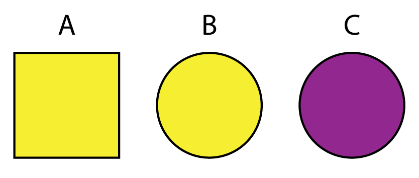
Boolean	Filter	Result
x	color == "yellow"	A, B
y	shape == "circle"	B, C
x & y	color == "yellow" & shape == "circle"	B
x | y	color == "yellow" | shape == "circle"	A, B, C
x & !y	color == "yellow" & shape != "circle"	A
!x & y	color != "yellow" & shape == "circle"	C
!(x & y)	!(color == "yellow" & shape == "circle")	A, C
!(x | y)	!(color == "yellow" | shape == "circle")	NULL

And here is an example with our penguins data, where we ask R to return those observations in which (a) penguins reside on Biscoe Island and (b) their bills are longer than 39 millimeters.

penguins |> filter(island == "Biscoe" & bill_length_mm > 39)

# A tibble: 143 × 8
   species island bill_length_mm bill_depth_mm flipper_len…¹ body_…² sex    year
   <fct>   <fct>           <dbl>         <dbl>         <int>   <int> <fct> <int>
 1 Adelie  Biscoe           40.6          18.6           183    3550 male   2007
 2 Adelie  Biscoe           40.5          17.9           187    3200 fema…  2007
 3 Adelie  Biscoe           40.5          18.9           180    3950 male   2007
 4 Adelie  Biscoe           39.6          17.7           186    3500 fema…  2008
 5 Adelie  Biscoe           40.1          18.9           188    4300 male   2008
 6 Adelie  Biscoe           42            19.5           200    4050 male   2008
 7 Adelie  Biscoe           41.4          18.6           191    3700 male   2008
 8 Adelie  Biscoe           40.6          18.8           193    3800 male   2008
 9 Adelie  Biscoe           41.3          21.1           195    4400 male   2008
10 Adelie  Biscoe           41.1          18.2           192    4050 male   2008
# … with 133 more rows, and abbreviated variable names ¹​flipper_length_mm,
#   ²​body_mass_g

Note that filter() let’s you separate conditions with a comma, which it interprets as conjunction, represented by the &.

penguins |> 
  filter(
    island == "Biscoe", 
    species == "Adelie", 
    body_mass_g < 3500
  )

# A tibble: 13 × 8
   species island bill_length_mm bill_depth_mm flipper_len…¹ body_…² sex    year
   <fct>   <fct>           <dbl>         <dbl>         <int>   <int> <fct> <int>
 1 Adelie  Biscoe           37.8          18.3           174    3400 fema…  2007
 2 Adelie  Biscoe           40.5          17.9           187    3200 fema…  2007
 3 Adelie  Biscoe           37.9          18.6           172    3150 fema…  2007
 4 Adelie  Biscoe           35            17.9           190    3450 fema…  2008
 5 Adelie  Biscoe           34.5          18.1           187    2900 fema…  2008
 6 Adelie  Biscoe           36.5          16.6           181    2850 fema…  2008
 7 Adelie  Biscoe           35.7          16.9           185    3150 fema…  2008
 8 Adelie  Biscoe           36.4          17.1           184    2850 fema…  2008
 9 Adelie  Biscoe           35.5          16.2           195    3350 fema…  2008
10 Adelie  Biscoe           37.7          16             183    3075 fema…  2009
11 Adelie  Biscoe           37.9          18.6           193    2925 fema…  2009
12 Adelie  Biscoe           38.1          17             181    3175 fema…  2009
13 Adelie  Biscoe           39.7          17.7           193    3200 fema…  2009
# … with abbreviated variable names ¹​flipper_length_mm, ²​body_mass_g

Exercises

1. Try all of the following with filter():
   • Filter penguins that reside on Torgersen island.
   • Filter penguins that have a flipper length greater than 185 mm.
   • Filter penguins that reside on Torgersen island and have a body mass less than 3500 g.

Groups

Your data will often include natural groupings (like species in the penguins table or dart types in the darts table), and you will want to summarize information about each of those groups. The way that you do this with dplyr involves the use of group_by() and summarize().

penguins |> group_by(species)

# A tibble: 344 × 8
# Groups:   species [3]
   species island    bill_length_mm bill_depth_mm flipper_…¹ body_…² sex    year
   <fct>   <fct>              <dbl>         <dbl>      <int>   <int> <fct> <int>
 1 Adelie  Torgersen           39.1          18.7        181    3750 male   2007
 2 Adelie  Torgersen           39.5          17.4        186    3800 fema…  2007
 3 Adelie  Torgersen           40.3          18          195    3250 fema…  2007
 4 Adelie  Torgersen           NA            NA           NA      NA <NA>   2007
 5 Adelie  Torgersen           36.7          19.3        193    3450 fema…  2007
 6 Adelie  Torgersen           39.3          20.6        190    3650 male   2007
 7 Adelie  Torgersen           38.9          17.8        181    3625 fema…  2007
 8 Adelie  Torgersen           39.2          19.6        195    4675 male   2007
 9 Adelie  Torgersen           34.1          18.1        193    3475 <NA>   2007
10 Adelie  Torgersen           42            20.2        190    4250 <NA>   2007
# … with 334 more rows, and abbreviated variable names ¹​flipper_length_mm,
#   ²​body_mass_g

Notice that the data are not changed, but the tibble now includes information about the groupings (Groups: species [3]). Now, if you apply summarize() to it, it will know that you want summaries for each group.

penguins |> 
  group_by(species) |> 
  summarize(
    mean_bill_length = mean(bill_length_mm, na.rm = TRUE),
    var_bill_length = var(bill_length_mm, na.rm = TRUE)
  )

# A tibble: 3 × 3
  species   mean_bill_length var_bill_length
  <fct>                <dbl>           <dbl>
1 Adelie                38.8            7.09
2 Chinstrap             48.8           11.2 
3 Gentoo                47.5            9.50

Note that you can summarize by multiple groups.

penguins |> 
  group_by(species, island) |> 
  summarize(
    mean_bill_length = mean(bill_length_mm, na.rm = TRUE),
    var_bill_length = var(bill_length_mm, na.rm = TRUE)
  )

# A tibble: 5 × 4
# Groups:   species [3]
  species   island    mean_bill_length var_bill_length
  <fct>     <fct>                <dbl>           <dbl>
1 Adelie    Biscoe                39.0            6.15
2 Adelie    Dream                 38.5            6.08
3 Adelie    Torgersen             39.0            9.15
4 Chinstrap Dream                 48.8           11.2 
5 Gentoo    Biscoe                47.5            9.50

A handy little function you will often want to use in summaries is n(). This counts the number of observations in each group.

penguins |> 
  group_by(species, island) |> 
  summarize(
    count = n(),
    mean_bill_length = mean(bill_length_mm, na.rm = TRUE),
    var_bill_length = var(bill_length_mm, na.rm = TRUE)
  )

# A tibble: 5 × 5
# Groups:   species [3]
  species   island    count mean_bill_length var_bill_length
  <fct>     <fct>     <int>            <dbl>           <dbl>
1 Adelie    Biscoe       44             39.0            6.15
2 Adelie    Dream        56             38.5            6.08
3 Adelie    Torgersen    52             39.0            9.15
4 Chinstrap Dream        68             48.8           11.2 
5 Gentoo    Biscoe      124             47.5            9.50

Now, suppose you wanted to get the three penguins in each species with the longest bills. To do that, you can apply the slice_max() function to the grouped penguins table.

penguins |> 
  group_by(species) |> 
  slice_max(bill_length_mm, n = 3)

# A tibble: 9 × 8
# Groups:   species [3]
  species   island    bill_length_mm bill_depth_mm flipper…¹ body_…² sex    year
  <fct>     <fct>              <dbl>         <dbl>     <int>   <int> <fct> <int>
1 Adelie    Torgersen           46            21.5       194    4200 male   2007
2 Adelie    Torgersen           45.8          18.9       197    4150 male   2008
3 Adelie    Biscoe              45.6          20.3       191    4600 male   2009
4 Chinstrap Dream               58            17.8       181    3700 fema…  2007
5 Chinstrap Dream               55.8          19.8       207    4000 male   2009
6 Chinstrap Dream               54.2          20.8       201    4300 male   2008
7 Gentoo    Biscoe              59.6          17         230    6050 male   2007
8 Gentoo    Biscoe              55.9          17         228    5600 male   2009
9 Gentoo    Biscoe              55.1          16         230    5850 male   2009
# … with abbreviated variable names ¹​flipper_length_mm, ²​body_mass_g

You can also get a random sample from each group (known as a stratified random sample) with slice_sample().

penguins |> 
  group_by(species) |> 
  slice_sample(n = 3)

# A tibble: 9 × 8
# Groups:   species [3]
  species   island bill_length_mm bill_depth_mm flipper_le…¹ body_…² sex    year
  <fct>     <fct>           <dbl>         <dbl>        <int>   <int> <fct> <int>
1 Adelie    Dream            42.3          21.2          191    4150 male   2007
2 Adelie    Biscoe           38.1          16.5          198    3825 fema…  2009
3 Adelie    Dream            36            17.9          190    3450 fema…  2007
4 Chinstrap Dream            48.5          17.5          191    3400 male   2007
5 Chinstrap Dream            52            20.7          210    4800 male   2008
6 Chinstrap Dream            51.3          19.9          198    3700 male   2007
7 Gentoo    Biscoe           48.4          14.6          213    5850 male   2007
8 Gentoo    Biscoe           46.4          15.6          221    5000 male   2008
9 Gentoo    Biscoe           45.2          16.4          223    5950 male   2008
# … with abbreviated variable names ¹​flipper_length_mm, ²​body_mass_g

Some other useful slice_*() functions include the following

• slice_head(n) takes the first n rows in each group.
• slice_tail(n) takes the last n rows in each group.
• slice_min(x, n) takes the n rows with the smallest values of x.
• slice_max(x, n) takes the n rows with the largest value of x.
• slice_sample(n) takes n random rows in each group.

Exercises

1. Group the penguins data by species and summarize the mean flipper length.
2. Group the penguins data by island and count the number of penguins on each. Hint: you can use n() to do this.
3. Group the penguins data by sex and summarize the mean and variance in body mass.
4. Group the penguins data by sex and species and summarize the mean and variance in body mass.
5. Group the darts data by type and summarize the mean length, width, and height.
6. Group the darts data by type and take a random sample of length five from each group.
7. Remove any potential duplicates from the darts data with distinct().